How accurately can you 1 predict Y from

For continuous type random variables (X, Y), the definitions of joint probability density function

Return to Class Exercise #1: Using the joint p. m. f. , E(X –

1. - continued Cov(X, Y) – 1 / 144 = ———————— X Y 35/144

2. Return - continued to Class Exercise #2: 1 Cov(X, Y) = E(XY) –

3. Return - continued to Class Exercise #3: 3 E(XY) = 3 3 (xy)

6. Return - continued to Class Exercise #6: f(x, y) f 1(x)f 2(y) Since

7. Return - continued to Class #7: Exercise E(XY) = 2 0 x 2

9. Return - continued to Class Exercise #9: f(x, y) f 1(x)f 2(y) Since

We let k(a, b) = E{[Y – (a + b. X)]2} = E{[(Y –

Note: A proof that – 1 1 is available by observing that all values

The least squares lines for predicting X from Y is 13 1 4 x

The least squares lines for predicting Y from X is 7 1 7 y

8. Return - continued to Class Exercise #8: f(x, y) = f 1(x)f 2(y)

The least squares lines for predicting Y from X is Since does not exist.

The least squares lines for predicting Y from X is 5 3 10 y

10. Suppose f 1(x) is the p. d. f. for the random variable X

(b) Show that Cov(X, Y) = XY = 0 if they exist. Cov(X, Y)

11. Suppose X has p. m. f. f 1(x) = 1/3 if x =

(c) Find the correlation between X and Y. E(X) = 0 Var(X) = 2/3

12. Suppose (X , Y) have joint p. d. f. f(x, y) = 1

(c) Find each of the following: The marginal p. d. f. of X is

12. - continued The marginal p. d. f. of Y is f 2(y) =

y 1 E(XY) = 0 xy dx dy = 0 –y Cov(X, Y) =

Name the distribution of a random variable which (a) is one if a specified

(l) can be changed into a standard normal random variable, when the mean of

13. Let X 1 and X 2 be any two random variables having finite

13. - continued (b) If the correlation between X 1 and X 2 is

Var(a 1 X 1 + a 2 X 2) = (using work done in

14. In doing each part of this exercise, note that the formulas derived in

Var(X – Y) = 2/3 + 2/9 = 8/9 E(2 X – 5 Y)

14. - continued (b) Let the random variables X and Y be as in

Var(X – Y) = 110/567 + 5/252 – 2(2/11)1/2(110/567)1/2(5/252)1/2 = 485/2268 – 20/378 =

14. - continued (c) Let the random variables X and Y be as in

(d) Let the random variables X and Y be as in Class Exercise #2.

15. - continued (b) Suppose that for any pair of distinct random variables Xi

Slides: 51

Download presentation

How accurately can you (1) predict Y from X, and (2) predict X from Y? 4/9 6 2/9 5 1/9 4 Y 1/9 3 1/9 2 1 1 2 3 4 X 5 6

How accurately can you (1) predict Y from X, and (2) predict X from Y? 6 5 1/12 4 1/6 1/6 3 1/12 Y 2 1 1 2 3 4 X 5 6

How accurately can you (1) predict Y from X, and (2) predict X from Y? 6 2/17 5 1/17 2/17 1/17 4 2/17 Y 1/17 3 2/17 1/17 2 2/17 1 1 2 3 4 X 5 2/17 6

How accurately can you (1) predict Y from X, and (2) predict X from Y? 6 5 1/5 4 Y 1/5 3 1/5 2 1/5 1 1 2 3 4 X 5 6

For continuous type random variables (X, Y), the definitions of joint probability density function (joint p. d. f. ), independence of X and Y, and mathematical expectation are each analogous to those for discrete type random variables, with summation signs replaced by integral signs. The covariance between random variables X and Y is Cov(X, Y) = E[(X – X)(Y – Y)] = E[XY – Y X – XY + X Y] = E(XY) – YE(X) – XE(Y) + X Y = E(XY) – X Y Cov(X, Y) The correlation between random variables X and Y is = ———— X Y Note: A proof that – 1 1 y will be available shortly. x

Return to Class Exercise #1: Using the joint p. m. f. , E(X – Y) = (1– 1)(1/6) + (1– 2)(1/4) + (2– 1)(1/4) + (2– 2)(1/3) = 0 Alternatively, E(X – Y) = 19/12 – 19/12 = 0 E(X + Y) can be interpreted as the mean of the total weight of candy in the bag. E(X – Y) can be interpreted as the mean of how much more the red candy in the bag weighs than the green candy. E(XY) = (1)(1)(1/6) + (1)(2)(1/4) + (2)(1)(1/4) + (2)(2)(1/3) = 5/2 1 Cov(X, Y) = E(XY) – E(X) E(Y) = (5/2) – (19/12) = – —— 144

1. - continued Cov(X, Y) – 1 / 144 = ———————— X Y 35/144 = The least squares lines for predicting Y from X is The least squares lines for predicting X from Y is 1 – — 35

2. Return - continued to Class Exercise #2: 1 Cov(X, Y) = E(XY) – E(X) E(Y) = (16/3) – (7/3) = – — 9 Cov(X, Y) – 1/9 1 = – — = ————— X Y 5/9 5 The least squares lines for predicting Y from X is The least squares lines for predicting X from Y is

3. Return - continued to Class Exercise #3: 3 E(XY) = 3 3 (xy) (xy / 36) = x=1 y=1 3 3 x=1 y=1 3 (xy) (x / 6) (y / 6) = x=1 y=1 (x) (x / 6) (y) (y / 6) = E(X) E(Y) = (7/3) = 49 / 9 Cov(X, Y) = E(XY) – E(X) E(Y) = (49/9) – (7/3) = 0 The least squares lines for predicting Y from X is The least squares lines for predicting X from Y is

6. Return - continued to Class Exercise #6: f(x, y) f 1(x)f 2(y) Since _____________, then the random variables X are not and Y ________ independent (as we previously noted). Using the joint p. m. f. , E(XY) = (1)(1)(1/6) + (3)(1)(1/6) + (2)(2)(1/6) + (3)(2)(1/6) + (2)(1)(1/3) = 3 1 Cov(X, Y) = E(XY) – E(X) E(Y) = 3 – (13/6)(4/3) = — 9 Cov(X, Y) 1/9 2 = ——————— = —— X Y 17 / 36 2 / 9 34 The least squares lines for predicting Y from X is

7. Return - continued to Class #7: Exercise E(XY) = 2 0 x 2 y + xy 2 ——— dx 8 xy f(x, y) dx dy = – – 2 2 0 2 2 x 3 y + 3 x 2 y 2 ————— dy = 48 x=0 0 dy = 0 2 2 4 y + 3 y 2 2 y 2 + y 3 4 ———— dy = ——— = — 12 12 3 y=0 1 Cov(X, Y) = E(XY) – E(X) E(Y) = 4/3 – (7/6) = – — 36 Cov(X, Y) – 1 / 36 1 = ———————— = – — 11 X Y 11 / 36

9. Return - continued to Class Exercise #9: f(x, y) f 1(x)f 2(y) Since _____________, then the random variables X are not and Y ________ independent (as we previously noted). 1 2 y 5 xy 2 E(XY) = xy f(x, y) dx dy = xy —— dx dy = 2 – – 0 0 1 2 y 1 1 1 2 y 5 x 2 y 3 5 x 3 y 3 20 y 6 20 y 7 20 —— dx dy = —— dy = —– = — 21 2 6 3 21 x=0 y=0 0 0 5 Cov(X, Y) = E(XY) – E(X) E(Y) = 20/21 – (10/9)(5/6) = —– 189 Cov(X, Y) 5 / 189 = ————————— = 2 / 11 X Y 110 / 567 5 / 252

We let k(a, b) = E{[Y – (a + b. X)]2} = E{[(Y – Y) – b(X – X) – (a – Y + b X)]2} = E[(Y – Y)2 + b 2(X – X)2 + (a – Y + b X)2 – 2 b(Y – Y)(X – X) – 2(Y – Y)(a – Y + b X) + 2 b(X – X)(a – Y + b X)] = Y 2 + b 2 X 2 + (a – Y + b X)2 – 2 b X Y – 2(0) + 2(0) = Y 2 + b 2 X 2 + (a – Y + b X)2 – 2 b X Y To minimize k(a, b) , we set the partial derivatives with respect to a and b equal to zero. (Note: This is textbook exercise 4. 2 -5. ) k — = 2(a – Y + b X) = 0 a k — = 2 b X 2 + 2(a – Y + b X) X – 2 X Y = 0 b (Multiply the first equation by X , subtract the resulting equation from the second equation, and solve for b. Then substitute in place of b in the first equation to solve for a. )

Note: A proof that – 1 1 is available by observing that all values of k(a, b), and in particular its minimum value, must be a nonnegative. Y b= — X Y a = Y – — X X The least squares line for predicting Y from X is Y Y y = Y – — X + — x X X The least squares line for predicting Y from X can be written y Y = Y + — (x – X) X The least squares line for predicting X from Y can be written x X = X + — (y – Y) Y Note that the point ( X , Y) is always on each of the least squares lines.

1. - continued Cov(X, Y) – 1 / 144 = ———————— X Y 35/144 1 – — 35 = The least squares lines for predicting Y from X is y 19 1 19 = — – — x – — 12 35 12 Y 1 35/144 1 b = — = – — ———— = – — X 35 35/144 35 The least squares lines for predicting X from Y is b = X 1 — = – — Y 35 x 19 1 19 = — – — y – — 12 35 12

2. Return - continued to Class Exercise #2: 1 Cov(X, Y) = E(XY) – E(X) E(Y) = (16/3) – (7/3) = – — 9 Cov(X, Y) – 1/9 1 = – — = ————— X Y 5/9 5 The least squares lines for predicting Y from X is y 7 1 7 = — – — x – — 3 5 3 x 7 1 7 = — – — y – — 3 5 3 Y 1 5/9 1 b = — = – — ——— = – — X 5 5/9 5 The least squares lines for predicting X from Y is b = X 1 — = – — Y 5

The least squares lines for predicting X from Y is 13 1 4 x = — + — y – — X 2 17 / 36 1 6 2 3 b = — = —— ———— = — Y 34 2/9 2 The conditional p. m. f. of Y | X = 1 is Y | X = 2 is Y | X = 3 is

The least squares lines for predicting Y from X is 7 1 7 y = — – — x – — 6 11 6 Y 1 11 / 36 1 b = — = – — ———— = – — X 11 / 36 11 The least squares lines for predicting X from Y is 7 1 7 x = — – — y – — 6 11 6 X 1 11 / 36 1 b = — = – — ———— = – — Y 11 / 36 11 For 0 < x < 2, the conditional p. d. f. of Y | X = x is

8. Return - continued to Class Exercise #8: f(x, y) = f 1(x)f 2(y) Since _____________, then the random variables X are and Y ________ independent 3 1 — x y– 1 xy —— dx dy = 2 x 2 E(XY) = 1 1 3 1 y 2 – y —— dy 2 dx = 1 7 — 3 Cov(X, Y) = = 1 — dx = x 1 Since E(XY) = , Cov(X, Y) and do not exist.

The least squares lines for predicting Y from X is Since does not exist. neither least The least squares lines for predicting X from Y is squares line exists. For 1 < x , the conditional p. d. f. of Y | X = x is For 1 < y < 3, the conditional p. d. f. of X | Y = y is For 1 < x , E(Y | X = x) = For 1 < x , Var(Y | X = x) = For 0 < y < 3, E(X | Y = y) = For 0 < y < 3, Var(X | Y = y) =

The least squares lines for predicting Y from X is 5 3 10 y = — + — x – — 6 22 9 Y 5 / 252 3 b = — = 2 / 11 ————— = — X 110 / 567 22 The least squares lines for predicting X from Y is 10 4 5 x = — + — y – — 9 3 6 X 110 / 567 4 4 b = — = 2 / 11 ————— = — =—y Y 5 / 252 3 3 For 0 < x < 2, the conditional p. d. f. of Y | X = x is

10. Suppose f 1(x) is the p. d. f. for the random variable X having space S 1 , suppose f 2(y) is the p. d. f. for the random variable Y having space S 2 , and suppose the joint p. d. f. for (X, Y) is f(x, y) = f 1(x)f 2(y) so that X and Y are independent. (a) Show that E[u 1(X) u 2(Y)] = E[u 1(X)] E[u 2(Y)] , if all expectations exist. E[u 1(X) u 2(Y)] = u 1(x) u 2(y) f 1(x) f 2(y) dx dy = S 1 S 2 u 2(y) f 2(y) S 2 u 1(x) f 1(x) dx dy = S 1 u 2(y) f 2(y) E[u 1(X)] dy = S 2 E[u 1(X)] u 2(y) f 2(y) dy = E[u 1(X)] E[u 2(Y)] S 2

(b) Show that Cov(X, Y) = XY = 0 if they exist. Cov(X, Y) = E(XY) – E(X) E(Y) = E(X) E(Y) – E(X) E(Y) = 0 which implies that X, Y = 0. (c) Explain why the results in parts (a) and (b) are still true when the p. d. f. s are replaced by p. m. f. s (that is, if X and Y are random variables of the discrete type instead of random variables of the continuous type). The integral signs in part (a) can be replaced with summation signs.

11. Suppose X has p. m. f. f 1(x) = 1/3 if x = – 1, 0, 1. Let Y = X 2 have p. m. f. f 2(y), and let f(x, y) be the joint p. m. f. for (X, Y). (a) Find the marginal p. m. f. of Y. The space of Y is {0, 1}. f 2(y) = (2/3)y(1/3)1–y if y = 0, 1 We recognize that Y has a Bernoulli(2/3) distribution. (b) Find and graphically display the space for (X, Y). Then find the joint p. m. f. for (X, Y). The space of (X, Y) is {(– 1, 1) (0, 0) (1, 1)}. 1 1/3 y 1/3 0 – 1 0 x 1 The joint p. m. f. of (X, Y) is f(x, y) = 1/3 if (x, y) = (– 1, 1) (0, 0) (1, 1)

(c) Find the correlation between X and Y. E(X) = 0 Var(X) = 2/3 E(Y) = 2/3 E(XY) = 0 Cov(X, Y) = E(XY) – E(X) E(Y) = 0 Var(Y) = 2/9 = 0 (d) Are X and Y independent? Does this answer depend on the value of (found in part (c))? X and Y cannot be independent, since the joint space is not “rectangular”. In fact, Y is totally determined by X. If X and Y were independent, then their correlation must be zero; however, when the correlation between two random variables is zero, the random variables may or may not be independent.

12. Suppose (X , Y) have joint p. d. f. f(x, y) = 1 if 0 < y < 1 , – y < x < y. (a) Graphically display the space for (X, Y). y (– 1, 1) (0, 0) x (b) Complete the following alternative description for the space for (X, Y): {(x, y) | – 1 < x < 0 , – x < y < 1 } {(x, y) | 0 < x < 1 , x < y < 1 }

(c) Find each of the following: The marginal p. d. f. of X is f 1(x) = Two separate f(x, y) dy = formulas needed 1+x if – 1 < x < 0 1–x if 0 < x < 1 – completing this exercise is homework! E(X) = – 1 0 1 x(1 + x) dx + 0 x(1 – x) dx = 0

12. - continued The marginal p. d. f. of Y is f 2(y) = 1 E(Y) = 0 2 y 2 dy = 2/3 2 y if 0 < y < 1

y 1 E(XY) = 0 xy dx dy = 0 –y Cov(X, Y) = E(XY) – E(X) E(Y) = 0 =0 (d) Are X and Y independent? Does this answer depend on the value of (found in part (c))? X and Y cannot be independent, since the joint space is not “rectangular”. If X and Y were independent, then their correlation must be zero; however, when the correlation between two random variables is zero, the random variables may or may not be independent.

Name the distribution of a random variable which (a) is one if a specified event occurs and zero otherwise. (b) is the number of times a specified event occurs in a set number of independent trials. (c) is the number of times a specified event occurs in a set number of trials which are not independent due to selection without replacement. (d) is the number of times a specified event occurs in an interval. (e) is the number of independent trials until a specified event occurs. (f) is the number of independent trials until a specified event occurs a set number of times. (g) is the length until a specified event occurs. (h) is the length until a specified event occurs a set number of times. (i) is a random number selected from an interval. (j) is the square of a standard normal random variable. (k) is a random number selected from the positive integers which are less than or equal to a set integer.

(l) can be changed into a standard normal random variable, when the mean of the distribution is subtracted and this difference divided by standard deviation of the distribution. (a) (b) (c) (d) (e) (f) (g) (h) (i) (j) (k) (l) Bernoulli distribution binomial distribution hypergeometric distribution Poisson distribution geometric distribution negative binomial distribution exponential distribution gamma distribution uniform distribution on the interval chi-square distribution with one degree of freedom uniform distribution on the first set number of positive integers any normal distribution

13. Let X 1 and X 2 be any two random variables having finite means and variances, with E(X 1) = 1 , E(X 2) = 2 , Var(X 1) = 12 , and Var(X 2) = 22. Let a 1 and a 2 be constants. (a) If X 1 and X 2 are independent, find each of the following: E(X 1 + X 2) = E(X 1) + E(X 2) = 1 + 2 E(a 1 X 1 + a 2 X 2) = E(a 1 X 1) + E(a 2 X 2) = a 1 E(X 1) + a 2 E(X 2) = a 1 1 + a 2 2 Var(X 1 + X 2) = E{[(X 1 + X 2) – ( 1 + 2)]2} = E{[(X 1 – 1) + (X 2 – 2)]2} = E{(X 1 – 1)2 + 2(X 1 – 1)(X 2 – 2) + (X 2 – 2)2} = E{(X 1 – 1)2} + 2 E{(X 1 – 1)(X 2 – 2)} + E{(X 2 – 2)2} = 12 + 2(0) + 22 = 12 + 22

Var(a 1 X 1 + a 2 X 2) = E{[(a 1 X 1 + a 2 X 2) – (a 1 1 + a 2 2)]2} = E{[a 1(X 1 – 1) + a 2(X 2 – 2)]2} = E{a 12 (X 1 – 1)2 + 2 a 1 a 2(X 1 – 1)(X 2 – 2) + a 22 (X 2 – 2)2} = a 12 E{(X 1 – 1)2} + 2 a 1 a 2 E{(X 1 – 1)(X 2 – 2)} + a 22 E{(X 2 – 2)2} = a 12 12 + 2 a 1 a 2(0) + a 22 22 = a 12 12 + a 22 22

13. - continued (b) If the correlation between X 1 and X 2 is 12 , find each of the following: E(X 1 + X 2) = E(X 1) + E(X 2) = 1 + 2 E(a 1 X 1 + a 2 X 2) = E(a 1 X 1) + E(a 2 X 2) = a 1 E(X 1) + a 2 E(X 2) = a 1 1 + a 2 2 Var(X 1 + X 2) = (using work done in part (a)) E{(X 1 – 1)2} + 2 E{(X 1 – 1)(X 2 – 2)} + E{(X 2 – 2)2} = 12 + 2 12 1 2 + 22 = 12 + 2 12 1 2

Var(a 1 X 1 + a 2 X 2) = (using work done in part (a)) a 12 E{(X 1 – 1)2} + 2 a 1 a 2 E{(X 1 – 1)(X 2 – 2)} + a 22 E{(X 2 – 2)2} = a 21 21 + 2 a 1 a 2 12 1 2 + a 22 22 = a 12 12 + a 22 22 + 2 a 1 a 2 12 1 2 (c) If the correlation between X 1 and X 2 is zero (0) but X 1 and X 2 are not independent, how are the formulas in part (a) affected? The formulas in part (a) remain the same if the correlation between X 1 and X 2 is zero (0), regardless of whether X 1 and X 2 are independent.

14. In doing each part of this exercise, note that the formulas derived in the previous exercise will be useful. (a) Let the random variables X and Y be as in Class Exercise #11. From calculations done in that exercise, complete the following: E(X) = 0 Var(X) = 2/3 E(Y) = 2/3 Var(Y) = 2/9 XY = 0 Use this information to find each of the following: E(X + Y) = 0 + 2/3 = 2/3 Var(X + Y) = 2/3 + 2/9 = 8/9 E(X – Y) = 0 – 2/3 = – 2/3

Var(X – Y) = 2/3 + 2/9 = 8/9 E(2 X – 5 Y) = 2(0) – 5(2/3) = – 10/3 Var(2 X – 5 Y) = 22(2/3) + (– 5)2(2/9) = 74/9

14. - continued (b) Let the random variables X and Y be as in Class Exercise #9. From calculations done in that exercise, complete the following: E(X) = 10/9 Var(X) = 110/567 E(Y) = 5/6 Var(Y) = 5/252 XY = 2 / 11 Use this information to find each of the following: E(X + Y) = 10/9 + 5/6 = 35/18 Var(X + Y) = 110/567 + 5/252 + 2(2/11)1/2(110/567)1/2(5/252)1/2 = 485/2268 + 10/189 = 605/2268 E(X – Y) = 10/9 – 5/6 = 5/18

Var(X – Y) = 110/567 + 5/252 – 2(2/11)1/2(110/567)1/2(5/252)1/2 = 485/2268 – 20/378 = 365/2268 E(2 X – 5 Y) = 2(10/9) – 5(5/6) = – 35/18 Var(2 X – 5 Y) = 22(110/567) + (– 5)2(5/252) + 2(2)(– 5)(2/11)1/2(110/567)1/2(5/252)1/2 = 2885/2268 – 200/378 = 1685/2268

14. - continued (c) Let the random variables X and Y be as in Class Exercise #3. From calculations done in that exercise, complete the following: E(X) = E(Y) = 7/3 Var(X) = Var(Y) = 5/9 XY = 0 Use this information to find each of the following: E(X + Y) = 7/3 + 7/3 = 14/3 Var(X + Y) = 5/9 + 5/9 = 10/9 E(X – Y) = 7/3 – 7/3 = 0 Var(X – Y) = 5/9 + 5/9 = 10/9 E(2 X – 5 Y) = 2(7/3) – 5(7/3) = – 7 Var(2 X – 5 Y) = 22(5/9) + (– 5)2(5/9) = 145/9

(d) Let the random variables X and Y be as in Class Exercise #2. From calculations done in that exercise, complete the following: E(X) = E(Y) = 7/3 Var(X) = Var(Y) = 5/9 XY = – 1/5 Use this information to find each of the following: E(X + Y) = 7/3 + 7/3 = 14/3 completing this exercise is homework! Var(X + Y) = 5/9 + 2(– 1/5)(5/9)1/2 = 8/9 E(X – Y) = 7/3 – 7/3 = 0 Var(X – Y) = 5/9 + 5/9 – 2(– 1/5)(5/9)1/2 = 4/3 E(2 X – 5 Y) = 2(7/3) – 5(7/3) = – 7 Var(2 X – 5 Y) = 22(5/9) + (– 5)2(5/9) + (2)(2)(– 5)(– 1/5)(5/9)1/2 = 165/9 = 55/3

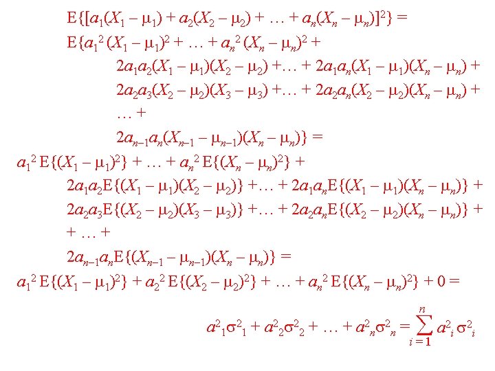
15. Let X 1 , X 2 , … , Xn be any n random variables having finite means and variances, with E(X 1) = 1 , E(X 2) = 2 , … , E(Xn) = n , Var(X 1) = 12 , Var(X 2) = 22 , …. Var(Xn) = n 2. Let a 1 , a 2 , … , an be constants and define the random variable n Y = a 1 X 1 + a 2 X 2 + … + an. Xn = ai Xi . i=1 (a) If X 1 , X 2 , … , Xn are (mutually) independent, find each of the following: E(Y) = E(a 1 X 1 + a 2 X 2 + … + an. Xn) = E(a 1 X 1) + E(a 2 X 2) + … + E(an. Xn) = a 1 E(X 1) + a 2 E(X 2) + … + an. E(Xn) = n a 1 1 + a 2 2 + … + an n = ai i i=1 Var(Y) = Var(a 1 X 1 + a 2 X 2 + … + an. Xn) = E{[(a 1 X 1 + a 2 X 2 + … + an. Xn) – (a 1 1 + a 2 2 + … + an n)]2} =

15. - continued (b) Suppose that for any pair of distinct random variables Xi and Xj , the correlation is ij ; then find each of the following: E(Y) = E(a 1 X 1 + a 2 X 2 + … + an. Xn) = (same as in part (a)) n a 1 1 + a 2 2 + … + an n = ai i i=1 Var(Y) = Var(a 1 X 1 + a 2 X 2 + … + an. Xn) = …(same as in part (a)) = a 12 E{(X 1 – 1)2} + … + an 2 E{(Xn – n)2} + 2 a 1 a 2 E{(X 1 – 1)(X 2 – 2)} +… + 2 a 1 an. E{(X 1 – 1)(Xn – n)} + 2 a 2 a 3 E{(X 2 – 2)(X 3 – 3)} +… + 2 a 2 an. E{(X 2 – 2)(Xn – n)} + +…+ 2 an– 1 an. E{(Xn– 1 – n– 1)(Xn – n)} =

n n– 1 n a 2 i 2 i + 2 i=1 i = 1 j = i +1 ai aj i j (c) Suppose that for any pair of distinct random variables Xi and Xj , the correlation is zero (0) but Xi and Xj may not be independent. How are the formulas in part (a) affected? The formulas in part (a) remain the same if the correlation between any pair Xi and Xj is zero (0), regardless of whether any pair Xi and Xj are independent.