Hmm HID HMMs Gerald Dalley MIT AI Lab

Hmm, HID HMMs Gerald Dalley MIT AI Lab Activity Perception Group Meeting 17 April 2003

Overview • • • The Problem HMM Background Binomial Field HMMs, a la Kale, et al. New Ideas

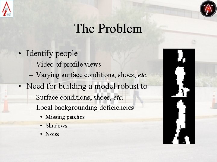
The Problem • Identify people – Video of profile views – Varying surface conditions, shoes, etc. • Need for building a model robust to – Surface conditions, shoes, etc. – Local backgrounding deficiencies • Missing patches • Shadows • Noise

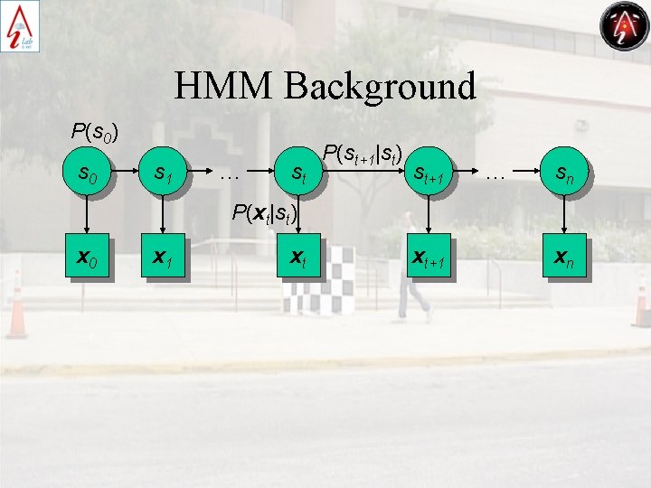
HMM Background P(s 0) s 0 s 1 … st P(st+1|st) st+1 … sn P(xt|st) x 0 x 1 xt xt+1 xn

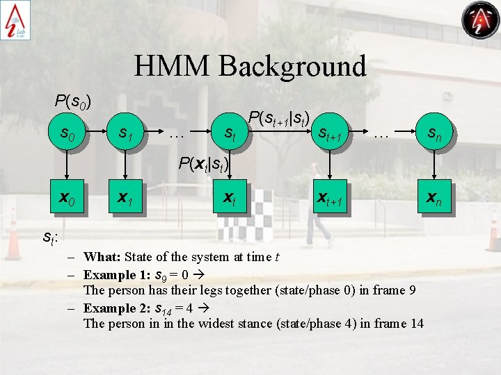
HMM Background P(s 0) s 0 s 1 … st P(st+1|st) st+1 … sn P(xt|st) x 0 st: x 1 xt xt+1 – What: State of the system at time t – Example 1: s 9 = 0 The person has their legs together (state/phase 0) in frame 9 – Example 2: s 14 = 4 The person in in the widest stance (state/phase 4) in frame 14 xn

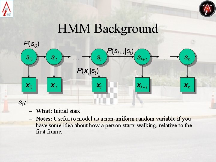
HMM Background P(s 0) s 0 s 1 … st P(st+1|st) st+1 … sn P(xt|st) x 0 s 0: x 1 xt xt+1 xn – What: Initial state – Notes: Useful to model as a non-uniform random variable if you have some idea about how a person starts walking, relative to the first frame.

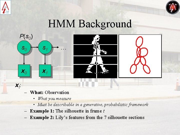
HMM Background P(s 0) s 0 s 1 x 0 x 1 xt : … – What: Observation • What you measure • Must be describable in a generative, probabilistic framework – Example 1: The silhouette in frame t – Example 2: Lily’s features from the 7 silhouette sections

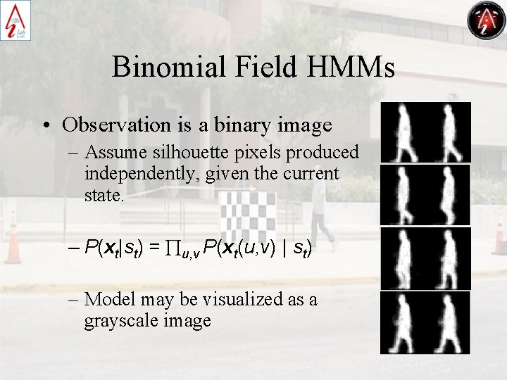
Binomial Field HMMs • Observation is a binary image – Assume silhouette pixels produced independently, given the current state. – P(xt|st) = Õu, v P(xt(u, v) | st) – Model may be visualized as a grayscale image

Some HMM Uses (one HMM person) • Make phase assignments • Help build an appearance model to clean up silhouettes – E. g. turn on any pixels in a silhouette when that pixel almost always is on given the most likely state assignment • Use directly for recognition – Determine the likelihood that each person’s HMM would generate a test sequence of silhouettes – Select the person most likely to generate the sequence

HMMs, a la Kale, et al. • Thought process – Independence is a bad assumption – Not enough data to learn even covariances – So, do a dimensionality reduction…

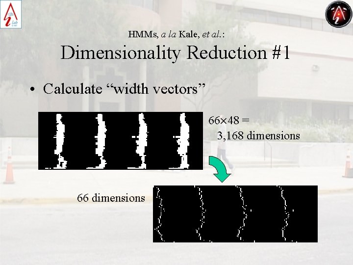
HMMs, a la Kale, et al. : Dimensionality Reduction #1 • Calculate “width vectors” 66£ 48 = 3, 168 dimensions 66 dimensions

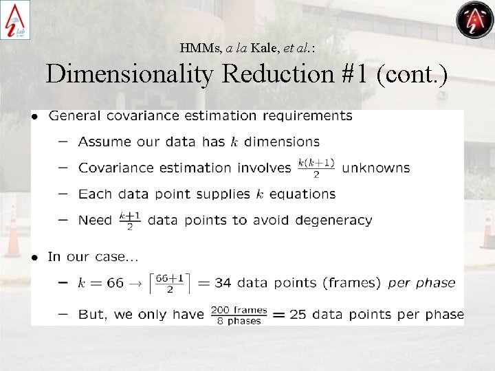
HMMs, a la Kale, et al. : Dimensionality Reduction #1 (cont. )

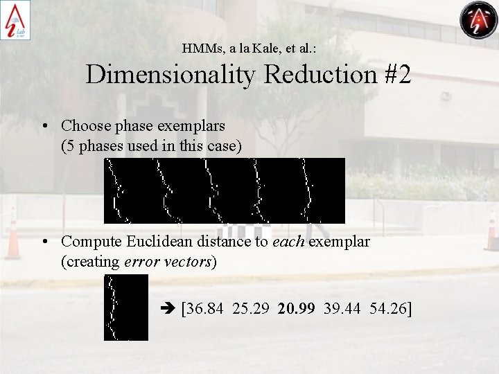
HMMs, a la Kale, et al. : Dimensionality Reduction #2 • Choose phase exemplars (5 phases used in this case) • Compute Euclidean distance to each exemplar (creating error vectors) [36. 84 25. 29 20. 99 39. 44 54. 26]

HMMs, a la Kale, et al. : Dimensionality Reduction #2 (cont. ) • Model error vectors as a joint Gaussian • For 8 phases, have ~5 equations for each unknown in the covariance

HMMs, a la Kale, et al. : Training • Estimate the walking period • Pick a set of equally-spaced frames from one period – “…we use the 5 stances which lead to minimum error in the 5 -d vector sequences. (in the sense of minimizing the norm). ” • Train the HMM – Update the mean and covariances of the error vectors – No updating of the exemplars…

HMMs, a la Kale, et al. : Training (cont. )

New Ideas • Cannot easily update exemplars in Kale’s approach, so… • Use projections onto “exemplars” instead of distances from them • Optimal “exemplars” are the PCA vectors

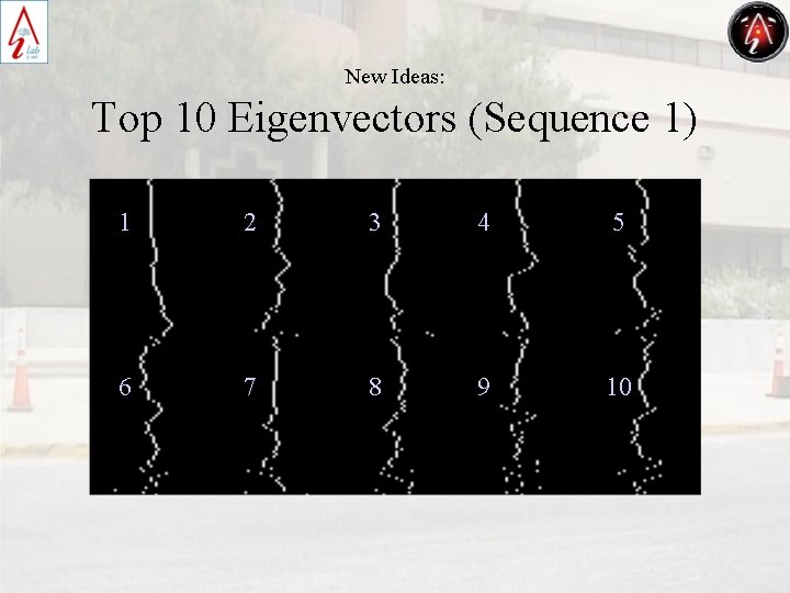
New Ideas: Top 10 Eigenvectors (Sequence 1) 1 2 3 4 5 6 7 8 9 10

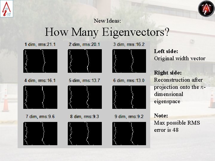
New Ideas: How Many Eigenvectors? Left side: Original width vector Right side: Reconstruction after projection onto the ndimensional eigenspace Note: Max possible RMS error is 48

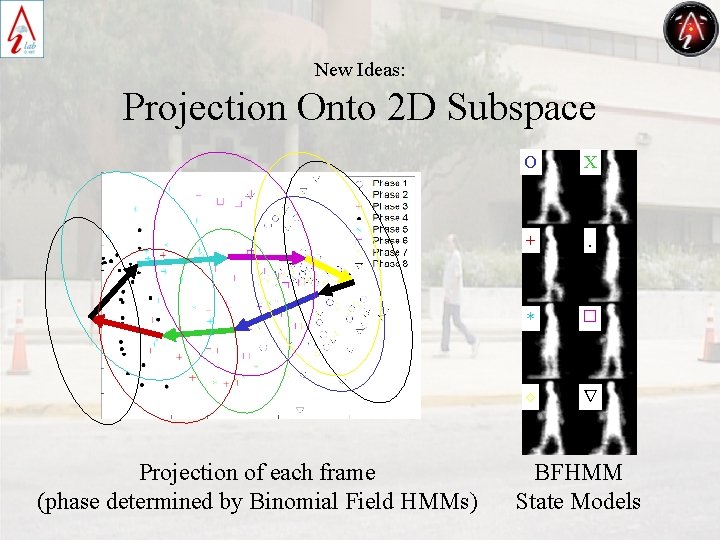
New Ideas: Projection Onto 2 D Subspace Projection of each frame (phase determined by Binomial Field HMMs) O X + . * ¤ ¦ r BFHMM State Models