histograms Mapping notation histograms Mapping notation 1 0

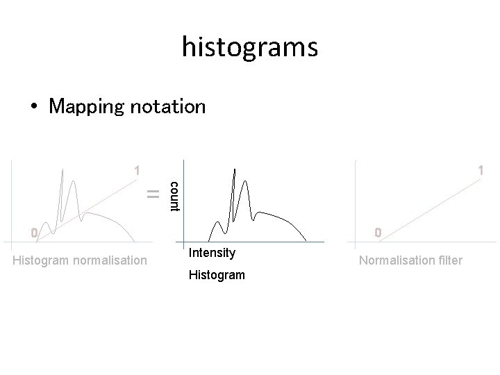
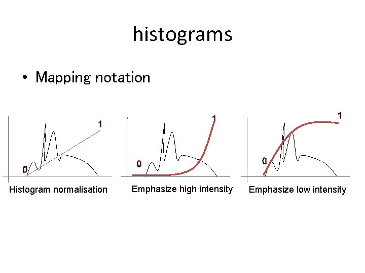
histograms • Mapping notation

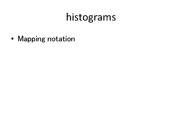
histograms • Mapping notation 1 0 Histogram normalisation

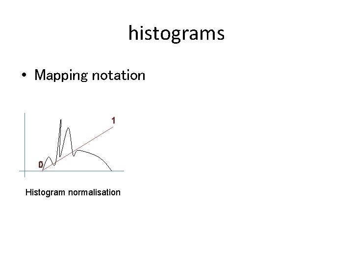
histograms • Mapping notation 1 1 = 0 0 Histogram normalisation Histogram Normalisation filter

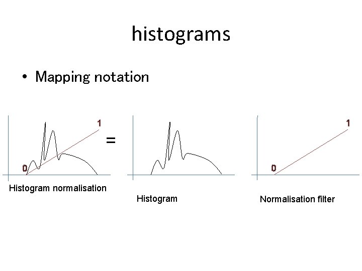
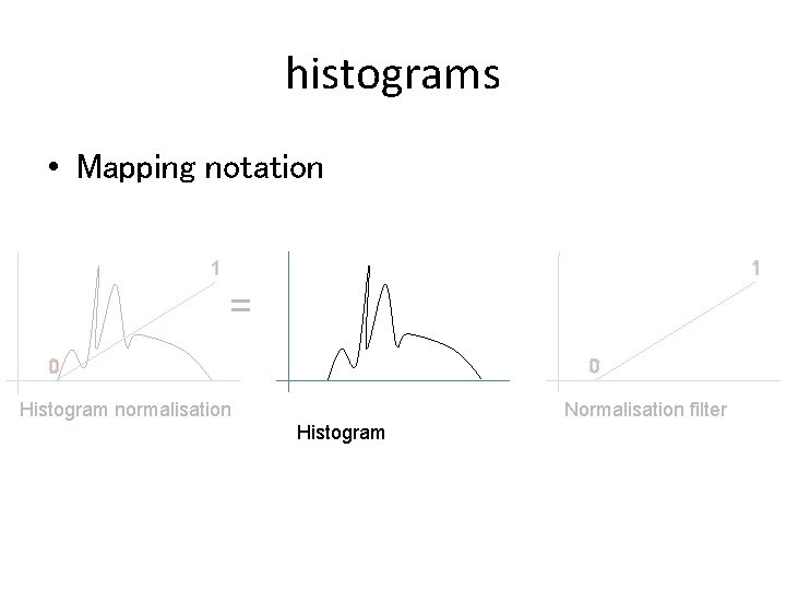
histograms • Mapping notation 1 1 = 0 0 Histogram normalisation Normalisation filter Histogram

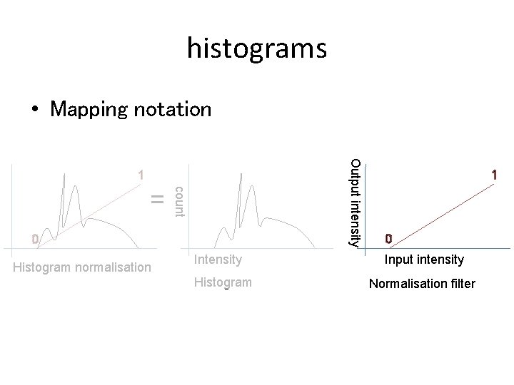
histograms • Mapping notation 1 1 count = 0 0 Histogram normalisation Intensity Histogram Normalisation filter

histograms • Mapping notation Output intensity 1 count = 0 Histogram normalisation Intensity Histogram 1 0 Input intensity Normalisation filter

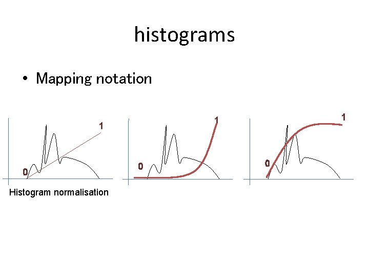
histograms • Mapping notation 1 0 Histogram normalisation 1 1 0 0

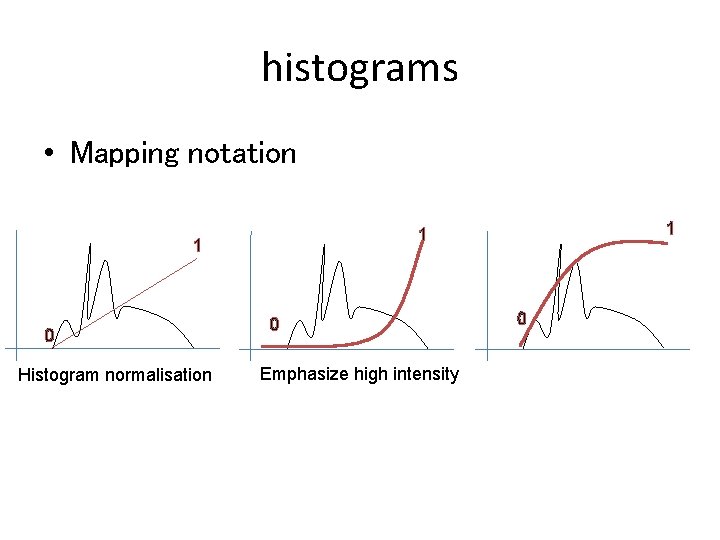
histograms • Mapping notation 1 0 Histogram normalisation 1 1 0 Emphasize high intensity 0

histograms • Mapping notation 1 0 Histogram normalisation 1 1 0 Emphasize high intensity 0 Emphasize low intensity

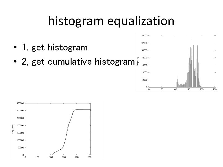
histogram equalization • 1, get histogram

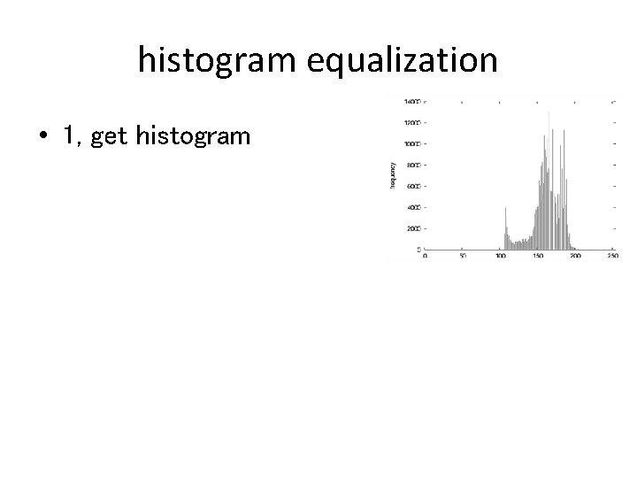
histogram equalization • 1, get histogram

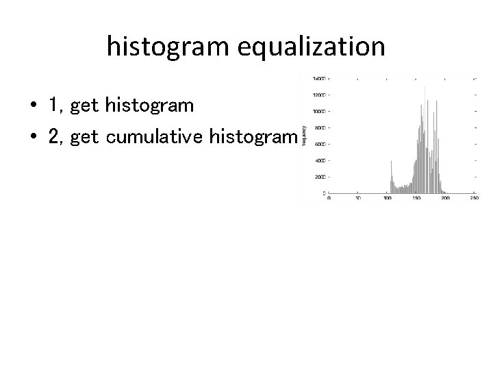
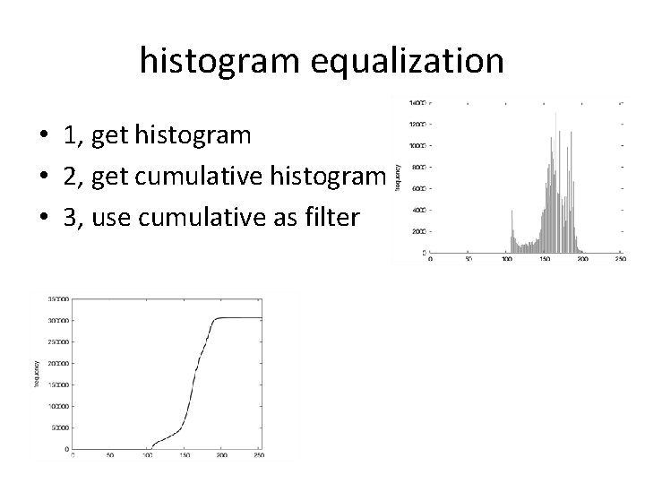
histogram equalization • 1, get histogram • 2, get cumulative histogram

histogram equalization • 1, get histogram • 2, get cumulative histogram

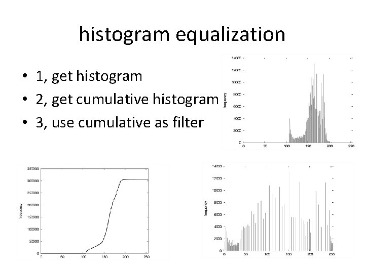
histogram equalization • 1, get histogram • 2, get cumulative histogram • 3, use cumulative as filter

histogram equalization • 1, get histogram • 2, get cumulative histogram • 3, use cumulative as filter

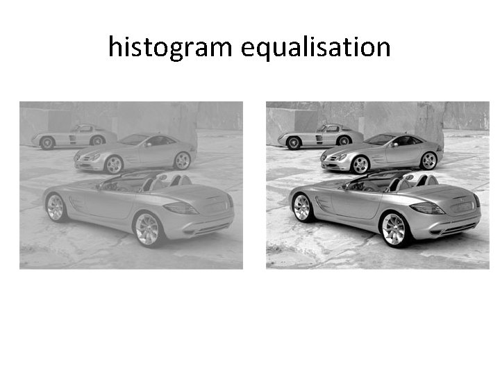
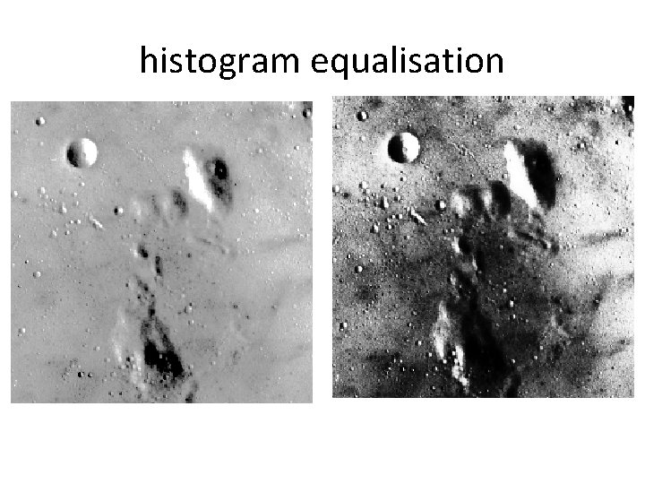
histogram equalisation

histogram equalisation

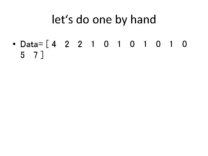
let‘s do one by hand • Data= [ 4 2 2 1 0 1 0 5 7]

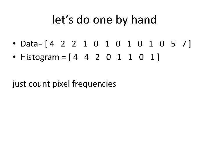
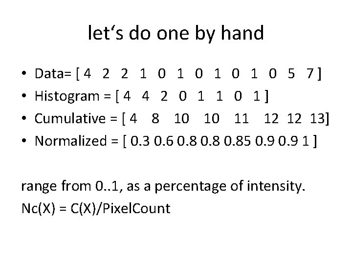
let‘s do one by hand • Data= [ 4 2 2 1 0 1 0 5 7 ] • Histogram = [ 4 4 2 0 1 1 0 1 ] just count pixel frequencies

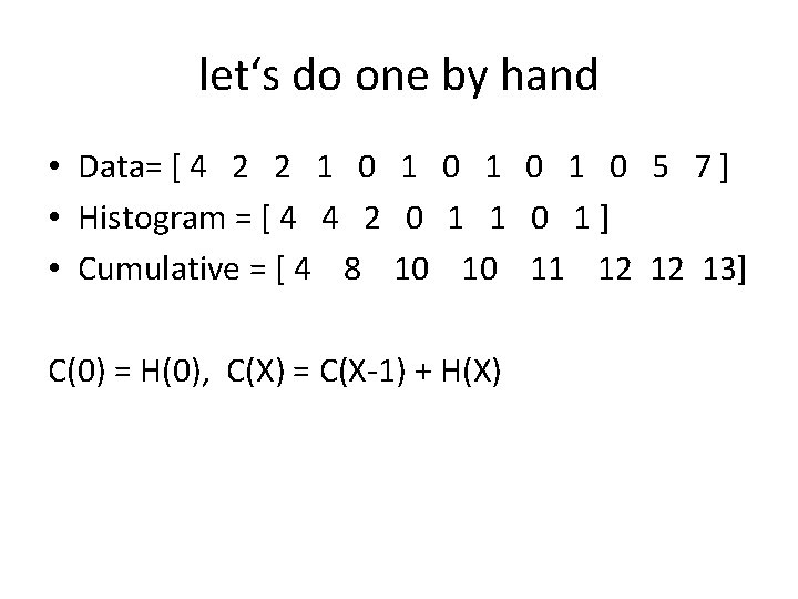
let‘s do one by hand • Data= [ 4 2 2 1 0 1 0 5 7 ] • Histogram = [ 4 4 2 0 1 1 0 1 ] • Cumulative = [ 4 8 10 10 11 12 12 13] C(0) = H(0), C(X) = C(X-1) + H(X)

let‘s do one by hand • • Data= [ 4 2 2 1 0 1 0 5 7 ] Histogram = [ 4 4 2 0 1 1 0 1 ] Cumulative = [ 4 8 10 10 11 12 12 13] Normalized = [ 0. 3 0. 6 0. 85 0. 9 1 ] range from 0. . 1, as a percentage of intensity. Nc(X) = C(X)/Pixel. Count

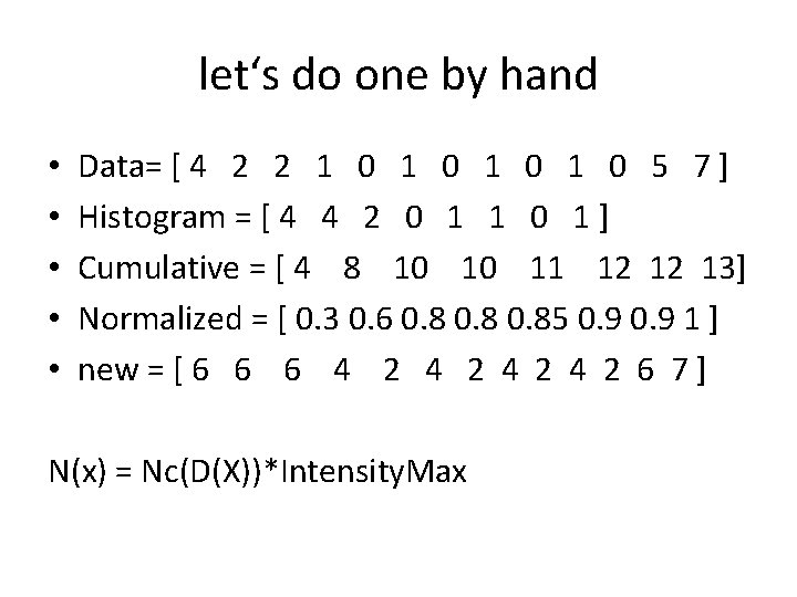
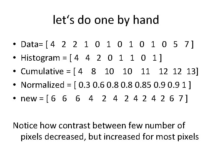
let‘s do one by hand • • • Data= [ 4 2 2 1 0 1 0 5 7 ] Histogram = [ 4 4 2 0 1 1 0 1 ] Cumulative = [ 4 8 10 10 11 12 12 13] Normalized = [ 0. 3 0. 6 0. 85 0. 9 1 ] new = [ 6 6 6 4 2 4 2 6 7 ] N(x) = Nc(D(X))*Intensity. Max

let‘s do one by hand • • • Data= [ 4 2 2 1 0 1 0 5 7 ] Histogram = [ 4 4 2 0 1 1 0 1 ] Cumulative = [ 4 8 10 10 11 12 12 13] Normalized = [ 0. 3 0. 6 0. 85 0. 9 1 ] new = [ 6 6 6 4 2 4 2 6 7 ] Notice how contrast between few number of pixels decreased, but increased for most pixels

practice • Do practice sheet • Email for solution, ill post it.

convolution kernels • Can do linear operations • 1) average

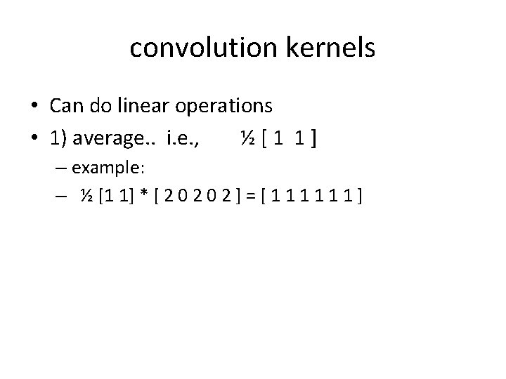
convolution kernels • Can do linear operations • 1) average. . i. e. , ½[1 1]

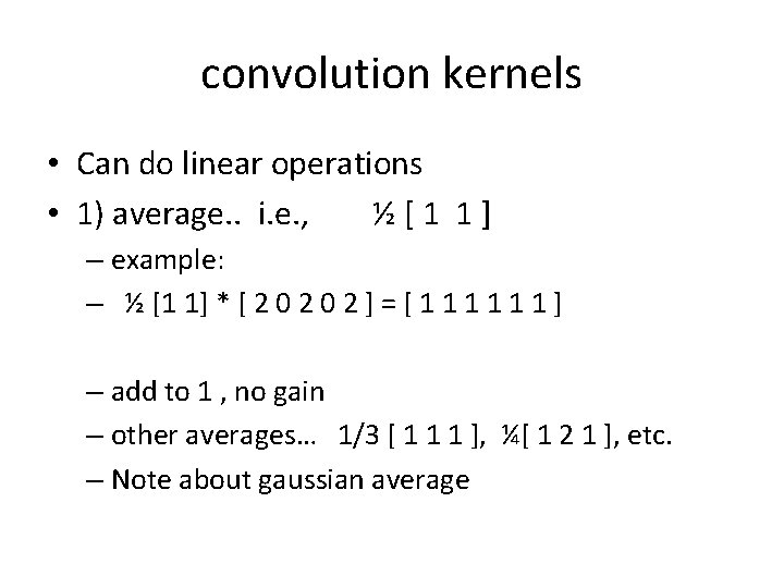
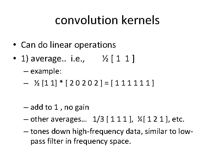
convolution kernels • Can do linear operations • 1) average. . i. e. , ½[1 1] – example: – ½ [1 1] * [ 2 0 2 ] = [ 1 1 1 ]

convolution kernels • Can do linear operations • 1) average. . i. e. , ½[1 1] – example: – ½ [1 1] * [ 2 0 2 ] = [ 1 1 1 ] – add to 1 , no gain – other averages… 1/3 [ 1 1 1 ], ¼[ 1 2 1 ], etc. – Note about gaussian average

convolution kernels • Can do linear operations • 1) average. . i. e. , ½[1 1] – example: – ½ [1 1] * [ 2 0 2 ] = [ 1 1 1 ] – add to 1 , no gain – other averages… 1/3 [ 1 1 1 ], ¼[ 1 2 1 ], etc. – tones down high-frequency data, similar to lowpass filter in frequency space.

convolution kernels • 2) derivative i. e. , [ 1 -1 ]

convolution kernels • 2) derivative i. e. , [ 1 -1 ] – Derived from calculus

convolution kernels • 2) derivative i. e. , [ 1 -1 ] – Derived from calculus – example: – [1 -1] * [ 1 2 3 4 5 6 ] = [ 1 1 1 -6 ]

convolution kernels • 2) derivative i. e. , [ 1 -1 ] – Derived from calculus – example: – [1 -1] * [ 1 2 3 4 5 6 ] = [ 1 1 1 -6 ] – Why does this find edges?

Examples!

move to 2 D • average: – Trivial. ¼ [1 1], or other extensions [1 1]

move to 2 D • derivative a little more complex. • Several varients. Next class.