Histograms and Color Balancing Empire of Light Magritte

Histograms and Color Balancing “Empire of Light”, Magritte Computational Photography Derek Hoiem, University of Illinois

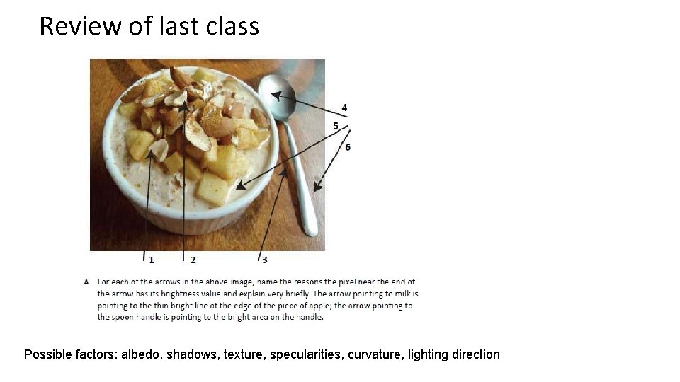
Review of last class Possible factors: albedo, shadows, texture, specularities, curvature, lighting direction

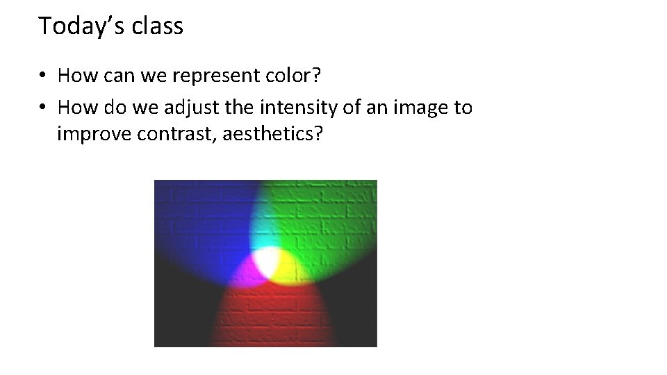
Today’s class • How can we represent color? • How do we adjust the intensity of an image to improve contrast, aesthetics?

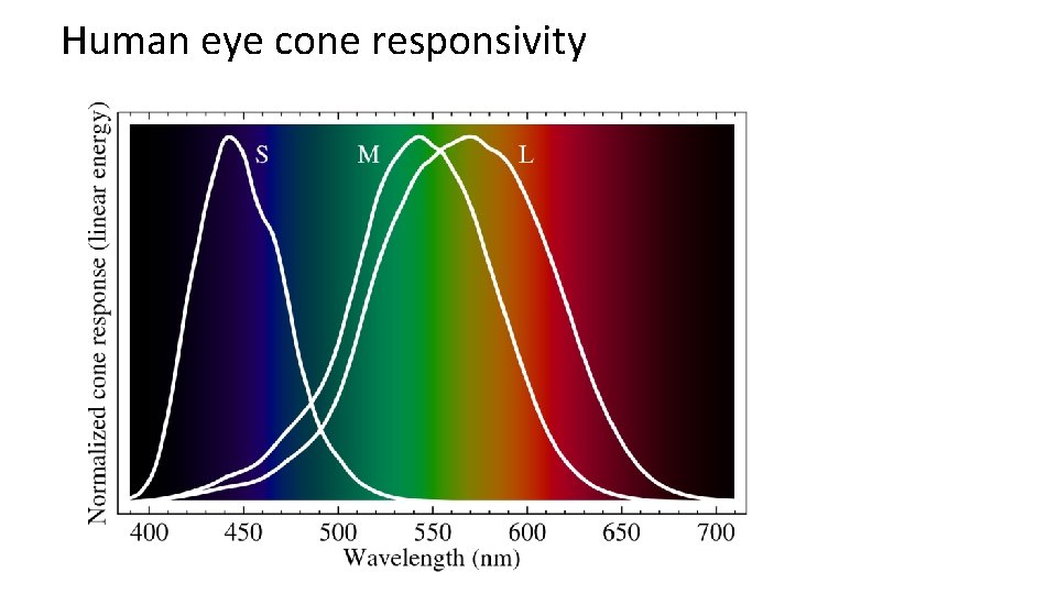
Human eye cone responsivity

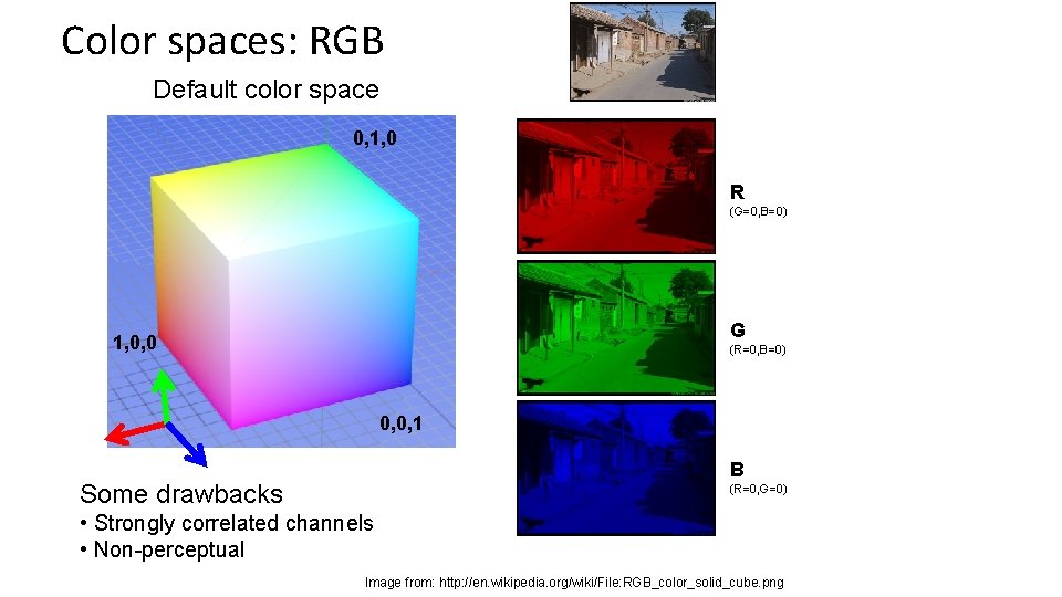
Color spaces: RGB Default color space 0, 1, 0 R (G=0, B=0) G 1, 0, 0 (R=0, B=0) 0, 0, 1 B Some drawbacks (R=0, G=0) • Strongly correlated channels • Non-perceptual Image from: http: //en. wikipedia. org/wiki/File: RGB_color_solid_cube. png

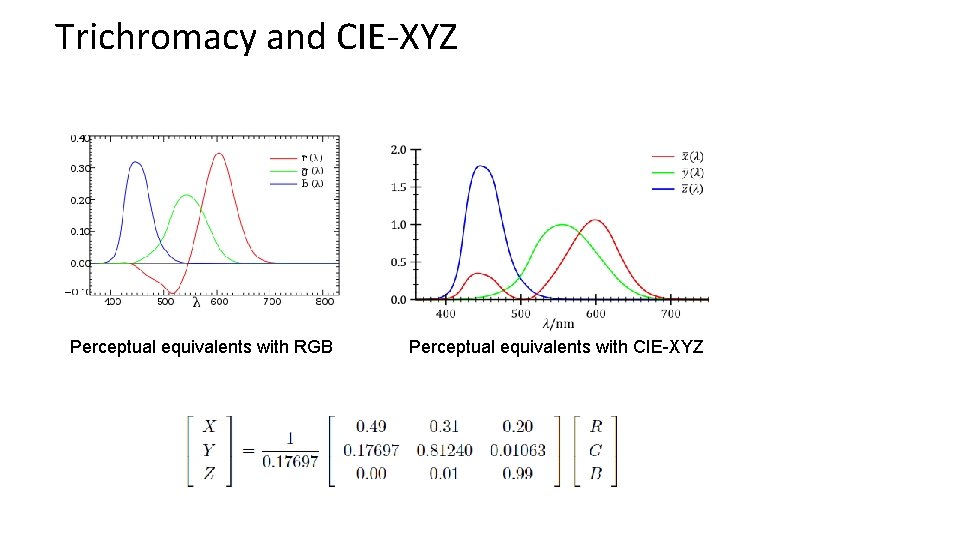
Trichromacy and CIE-XYZ Perceptual equivalents with RGB Perceptual equivalents with CIE-XYZ

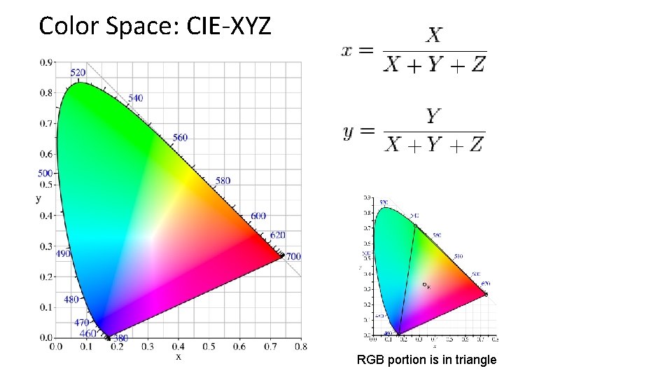
Color Space: CIE-XYZ RGB portion is in triangle

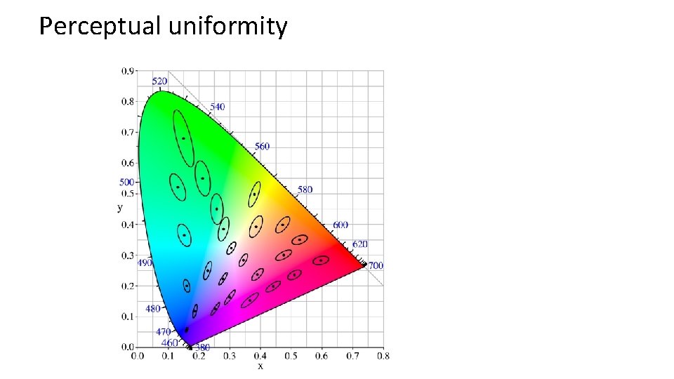
Perceptual uniformity

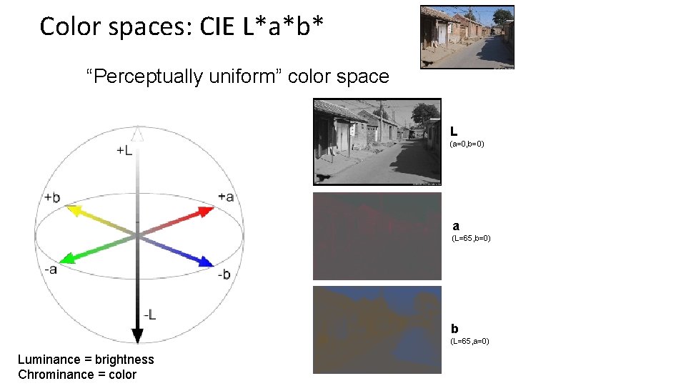
Color spaces: CIE L*a*b* “Perceptually uniform” color space L (a=0, b=0) a (L=65, b=0) b (L=65, a=0) Luminance = brightness Chrominance = color

If you had to choose, would you rather go without luminance or chrominance?

If you had to choose, would you rather go without luminance or chrominance?

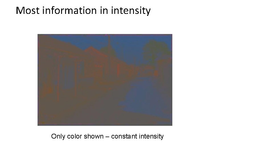
Most information in intensity Only color shown – constant intensity

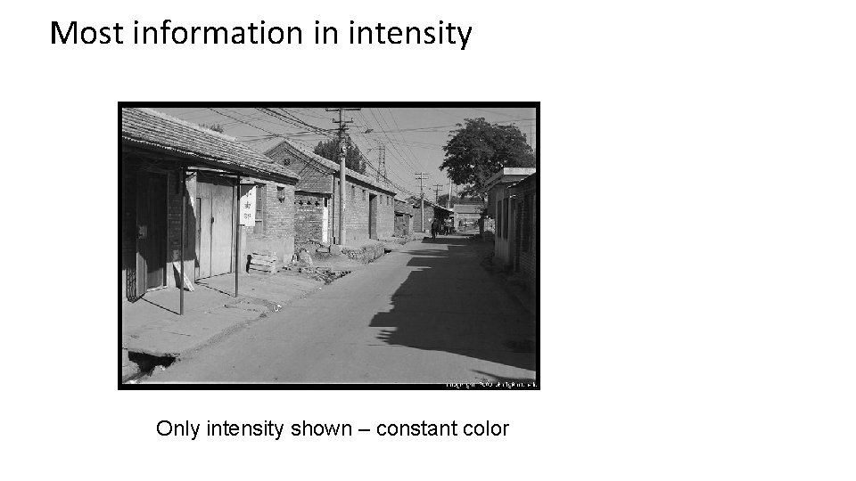
Most information in intensity Only intensity shown – constant color

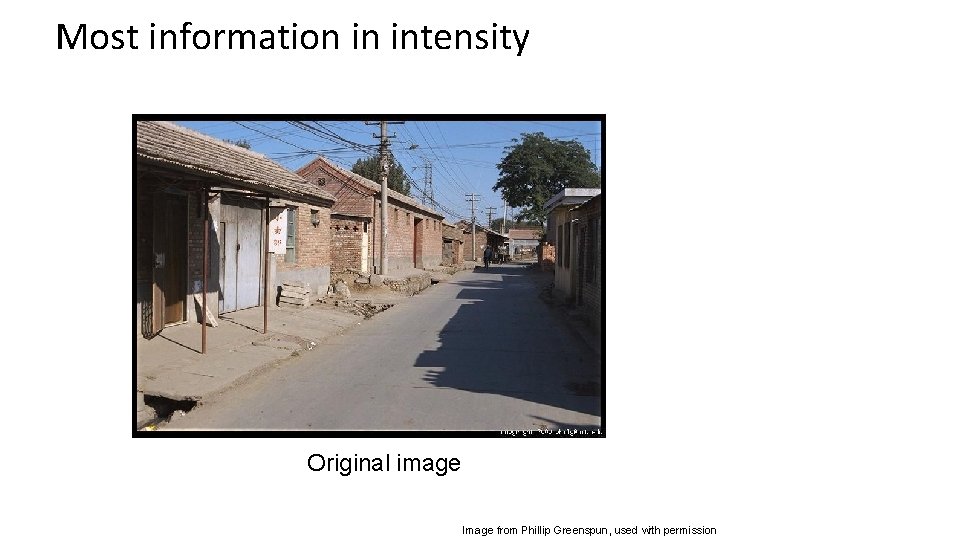
Most information in intensity Original image Image from Phillip Greenspun, used with permission

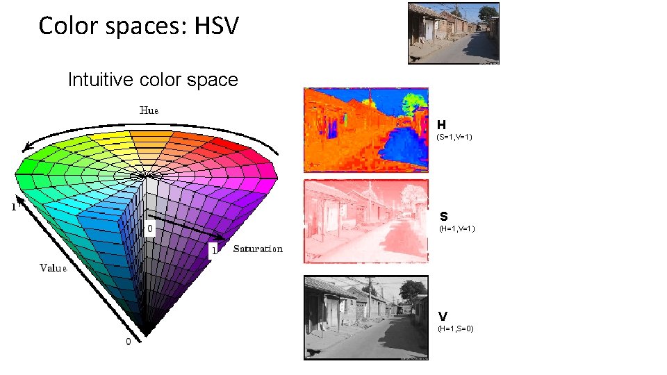
Color spaces: HSV Intuitive color space H (S=1, V=1) S (H=1, V=1) V (H=1, S=0)

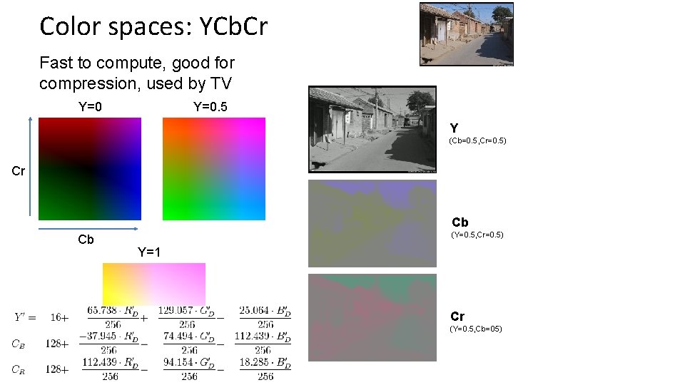
Color spaces: YCb. Cr Fast to compute, good for compression, used by TV Y=0. 5 Y (Cb=0. 5, Cr=0. 5) Cr Cb Cb (Y=0. 5, Cr=0. 5) Y=1 Cr (Y=0. 5, Cb=05)

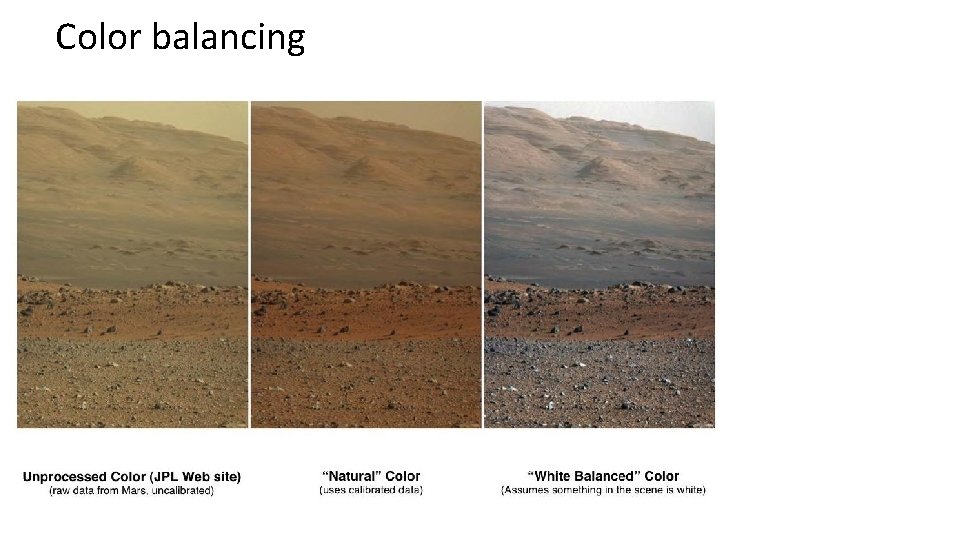
Color balancing

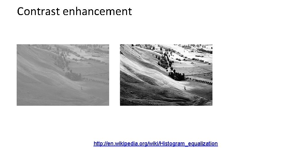
Contrast enhancement http: //en. wikipedia. org/wiki/Histogram_equalization

Important ideas • Typical images are gray on average; this can be used to detect distortions • Larger differences are more visible, so using the full intensity range improves visibility • It’s often easier to work in a non-RGB color space

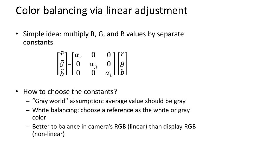
Color balancing via linear adjustment •

Tone Mapping • Typical problem: compress values from a high range to a smaller range – E. g. , camera captures 12 -bit linear intensity and needs to compress to 8 bits

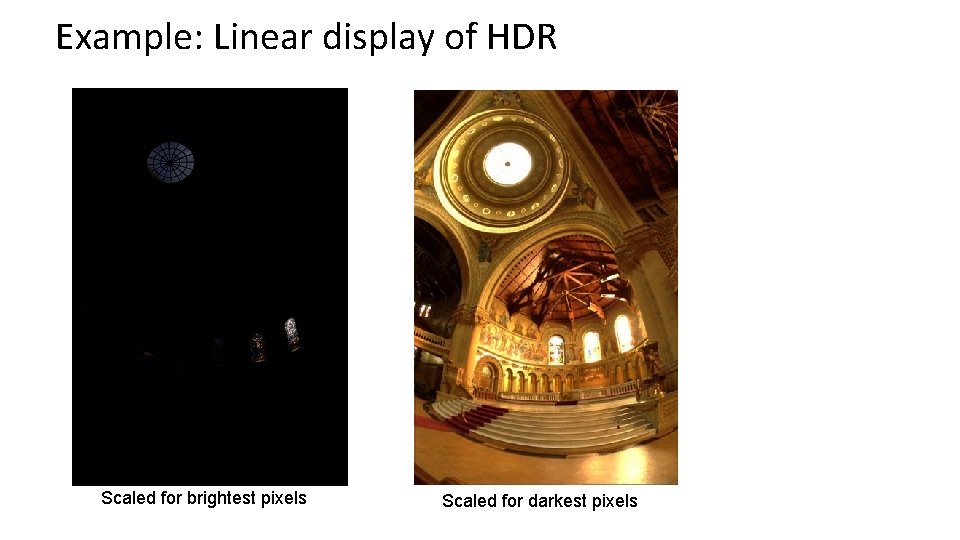
Example: Linear display of HDR Scaled for brightest pixels Scaled for darkest pixels

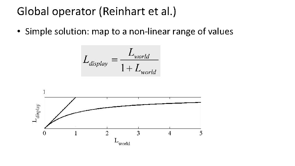
Global operator (Reinhart et al. ) • Simple solution: map to a non-linear range of values

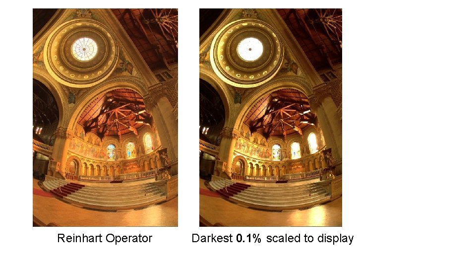
Reinhart Operator Darkest 0. 1% scaled to display

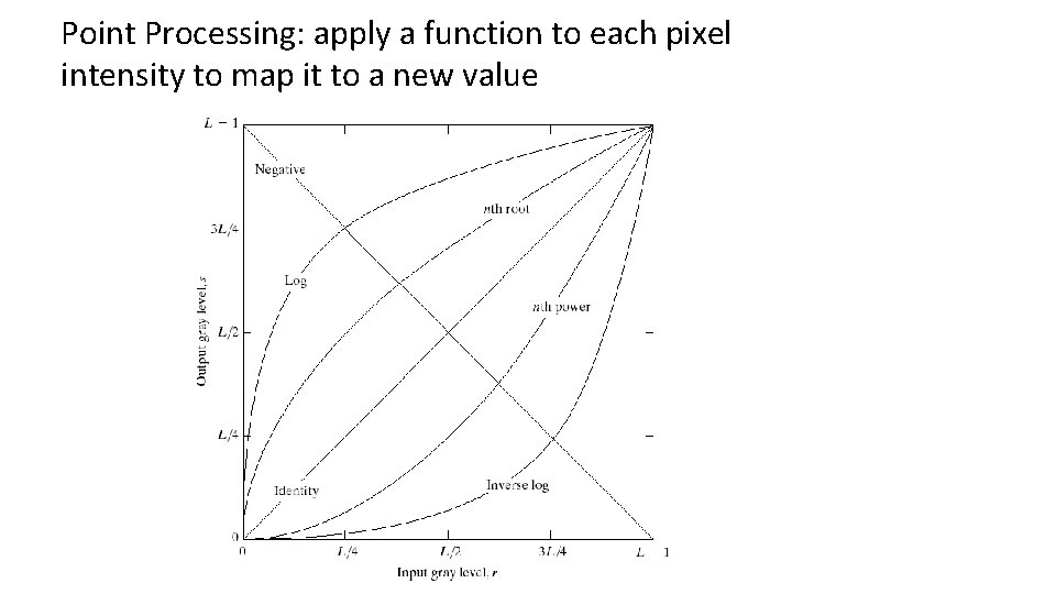
Point Processing: apply a function to each pixel intensity to map it to a new value

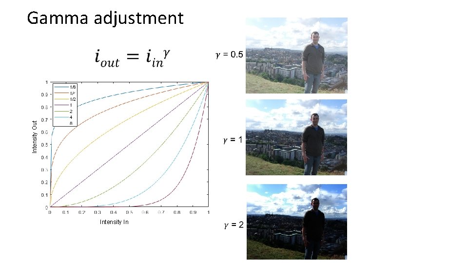
Intensity Out Gamma adjustment Intensity In

Matlab example

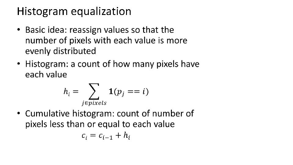
Histogram equalization •

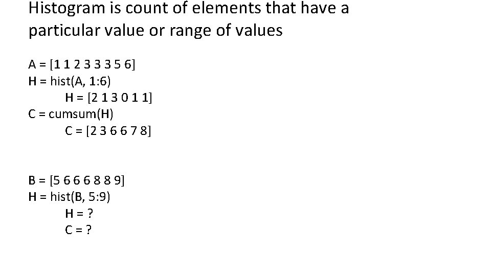
Histogram is count of elements that have a particular value or range of values A = [1 1 2 3 3 3 5 6] H = hist(A, 1: 6) H = [2 1 3 0 1 1] C = cumsum(H) C = [2 3 6 6 7 8] B = [5 6 6 6 8 8 9] H = hist(B, 5: 9) H=? C=?

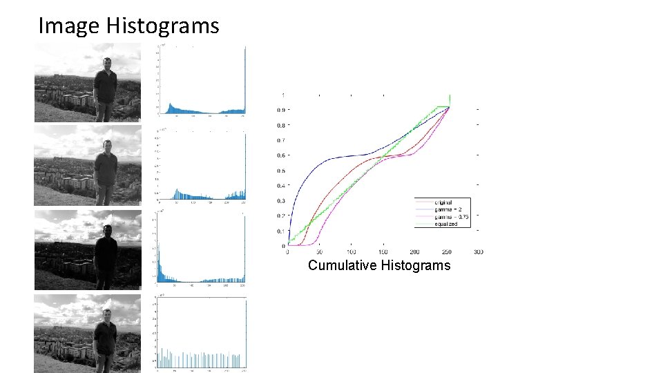
Image Histograms Cumulative Histograms

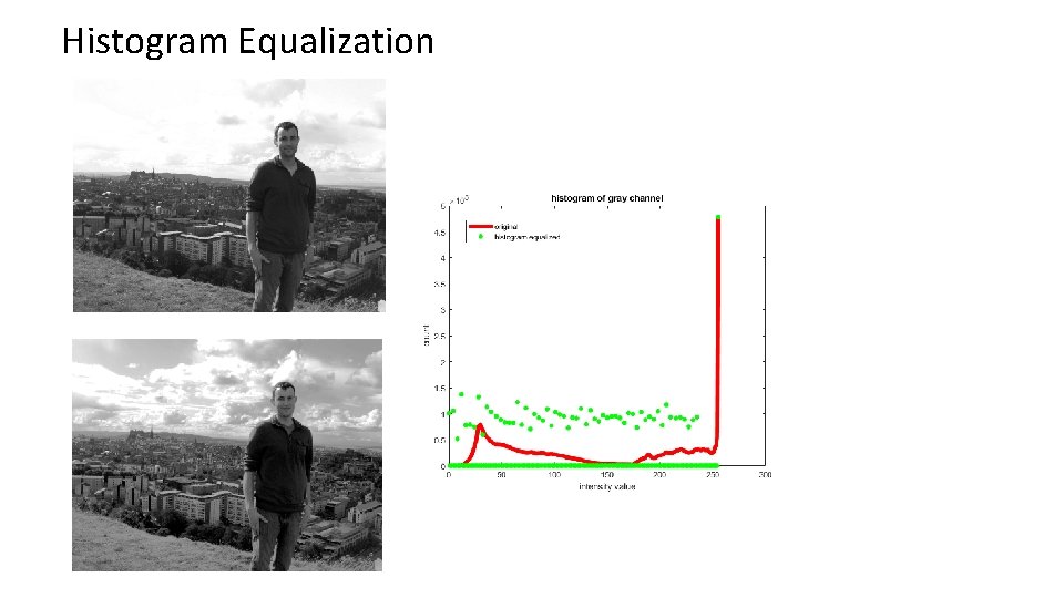
Histogram Equalization

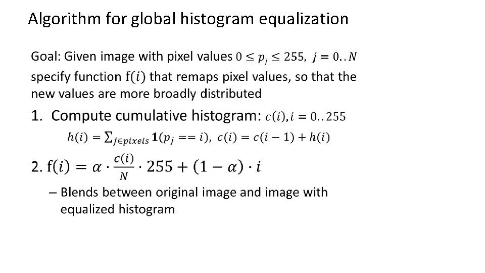
Algorithm for global histogram equalization •

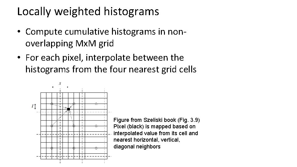
Locally weighted histograms • Compute cumulative histograms in nonoverlapping Mx. M grid • For each pixel, interpolate between the histograms from the four nearest grid cells Figure from Szeliski book (Fig. 3. 9) Pixel (black) is mapped based on interpolated value from its cell and nearest horizontal, vertical, diagonal neighbors

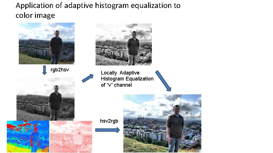
Application of adaptive histogram equalization to color image rgb 2 hsv Locally Adaptive Histogram Equalization of “v” channel hsv 2 rgb

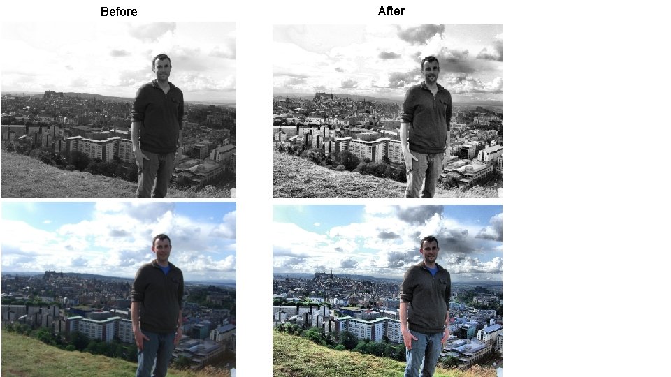
Before After

Other issues • Dealing with color images – Often better to split into luminance and chrominance to avoid unwanted color shift • Manipulating particular regions – Can use mask to select particular areas for manipulation • Useful Python functions/modules – skimage. color: color conversion, e. g. rgb 2 hsv – numpy: histogram, cumsum

Matlab Example 2

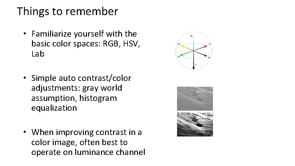
Things to remember • Familiarize yourself with the basic color spaces: RGB, HSV, Lab • Simple auto contrast/color adjustments: gray world assumption, histogram equalization • When improving contrast in a color image, often best to operate on luminance channel

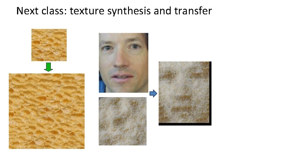
Next class: texture synthesis and transfer