HIRLAM coupled to the ocean wave model WAM

HIRLAM coupled to the ocean wave model WAM. Verification and improvements in forecast skill. Morten Ødegaard Køltzow, Øyvind Sætra and Ana Carrasco. The Norwegian Meteorological Institute

Outline: • Motivation. • What was the conclusions a year ago? • What is new this year? • Conclusions.

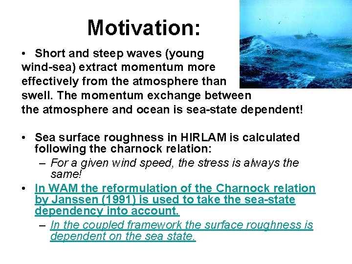
Motivation: • Short and steep waves (young wind-sea) extract momentum more effectively from the atmosphere than swell. The momentum exchange between the atmosphere and ocean is sea-state dependent! • Sea surface roughness in HIRLAM is calculated following the charnock relation: – For a given wind speed, the stress is always the same! • In WAM the reformulation of the Charnock relation by Janssen (1991) is used to take the sea-state dependency into account. – In the coupled framework the surface roughness is dependent on the sea state.

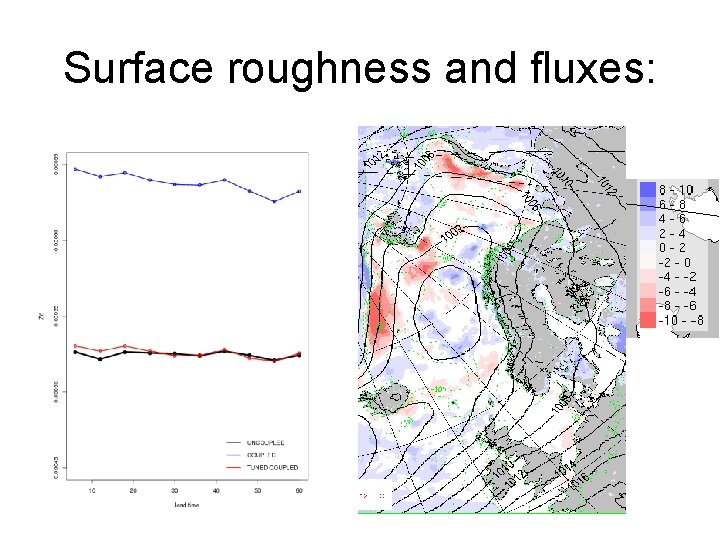
Summary Brussels 2008: • HIRLAM coupled to the wave model WAM and an experiment over 3 winter months had been performed. • An increased (~20%) roughness length over the ocean was found, with increased release of sensible heat and decreased release of latent heat. • Only minor impacts on the general performance of the model system (standard verification of MSLP, FF 10 m, T 2 m and precipitation). – Can this be improved by a tuning of the roughness length to keep the domain average of it constant? • An (possibly positive) impact on simulating Polar Lows is found.

The last year: • A tuned experiment: – Z 0 = constant x Z 0. – Since HIRLAM is a well tuned model we want to that the friction on average for the integration domain is not changed, but only re-distributed between young wind sea and swell. • Studied the sensitivity to initial conditions for the forecast of one polar low. • Experiments with HIRLAM coupled to WAM in the Norwegian LAMEPS system. • More detailed analysis.

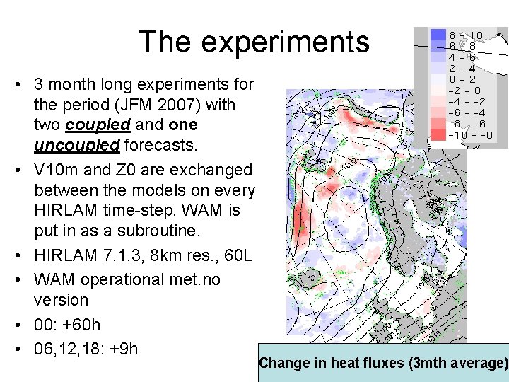
The experiments • 3 month long experiments for the period (JFM 2007) with two coupled and one uncoupled forecasts. • V 10 m and Z 0 are exchanged between the models on every HIRLAM time-step. WAM is put in as a subroutine. • HIRLAM 7. 1. 3, 8 km res. , 60 L • WAM operational met. no version • 00: +60 h • 06, 12, 18: +9 h Change in heat fluxes (3 mth average)

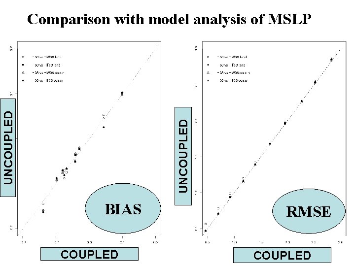
UNCOUPLED Comparison with model analysis of MSLP BIAS COUPLED RMSE COUPLED

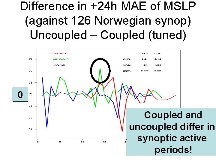
Difference in +24 h MAE of MSLP (against 126 Norwegian synop) Uncoupled – Coupled (tuned) 0 Coupled and uncoupled differ in synoptic active periods!

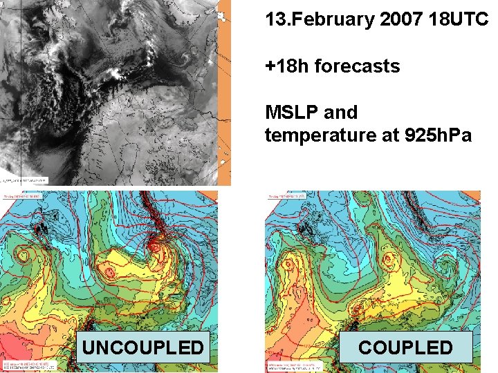
13. February 2007 18 UTC +18 h forecasts MSLP and temperature at 925 h. Pa UNCOUPLED

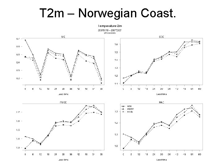
T 2 m – Norwegian Coast.

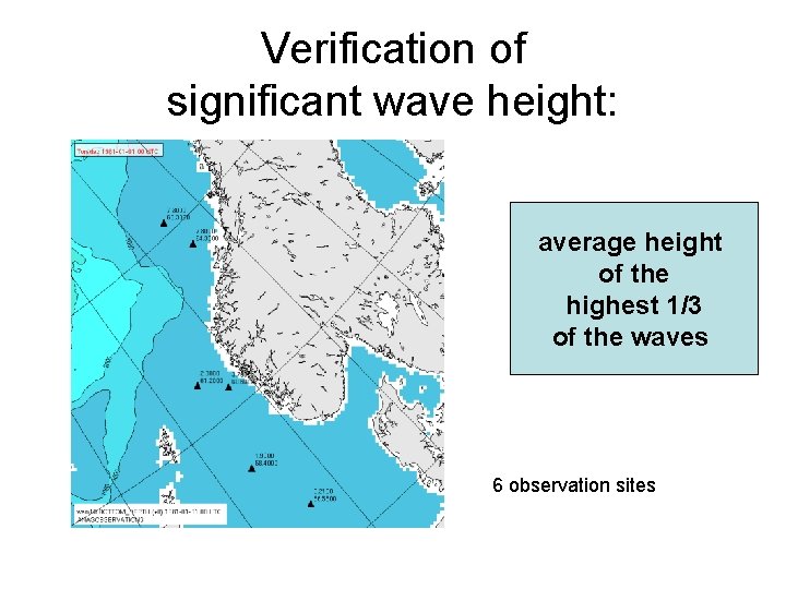
Verification of significant wave height: average height of the highest 1/3 of the waves 6 observation sites

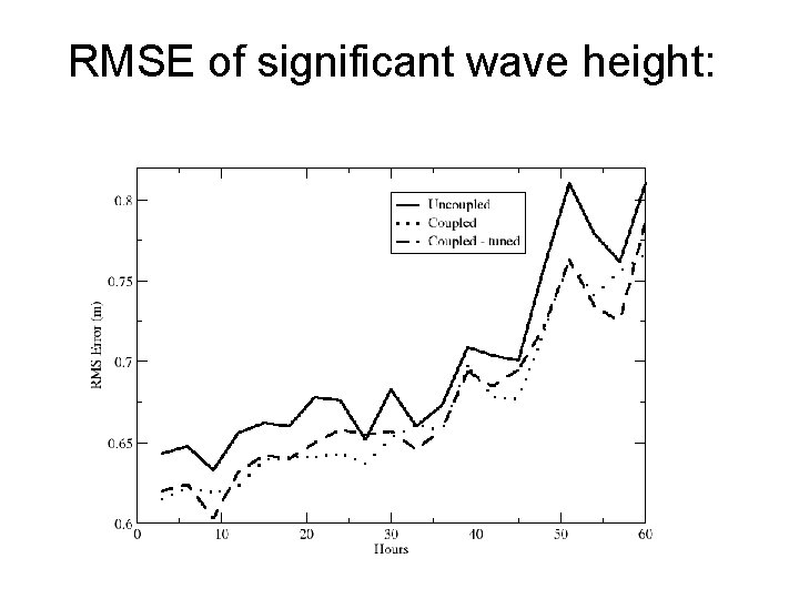
RMSE of significant wave height:

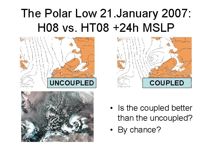
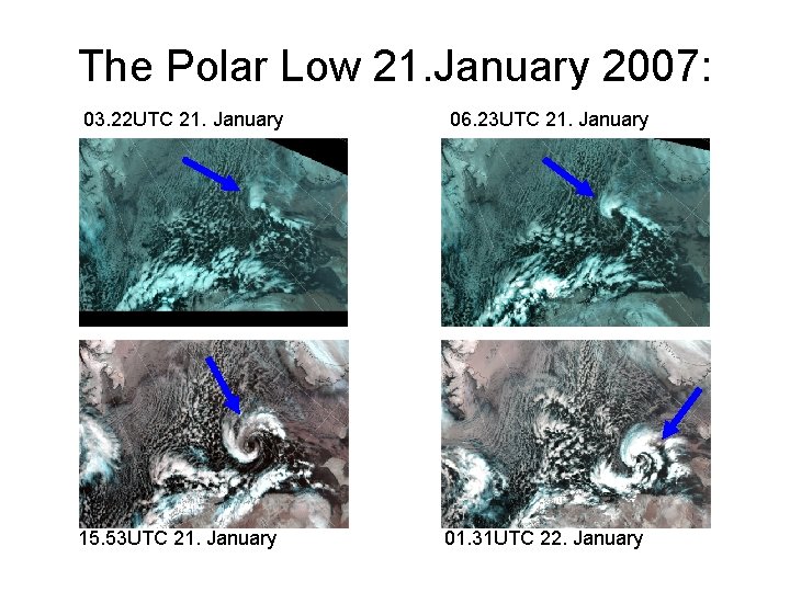
The Polar Low 21. January 2007: H 08 vs. HT 08 +24 h MSLP UNCOUPLED • Is the coupled better than the uncoupled? • By chance?

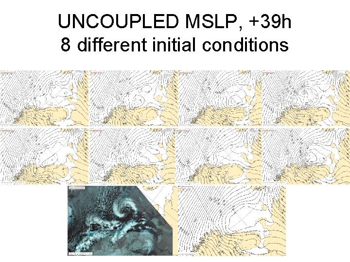
UNCOUPLED MSLP, +39 h 8 different initial conditions

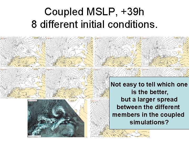
Coupled MSLP, +39 h 8 different initial conditions. Not easy to tell which one is the better, but a larger spread between the different members in the coupled simulations?

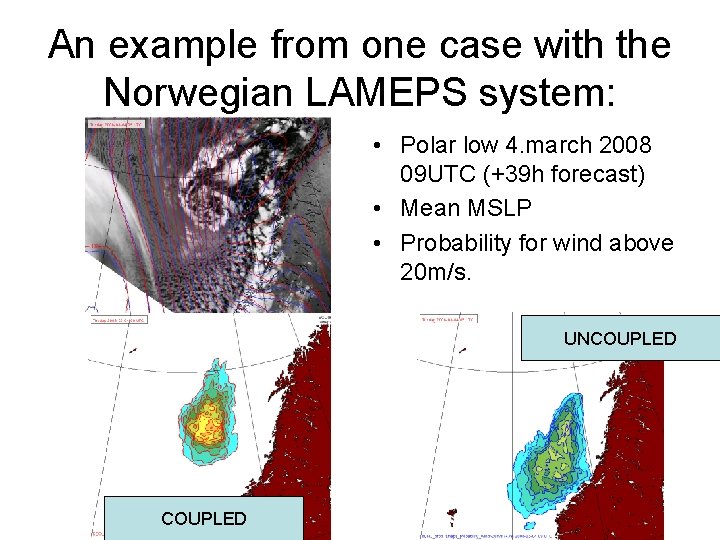
An example from one case with the Norwegian LAMEPS system: • Polar low 4. march 2008 09 UTC (+39 h forecast) • Mean MSLP • Probability for wind above 20 m/s. UNCOUPLED

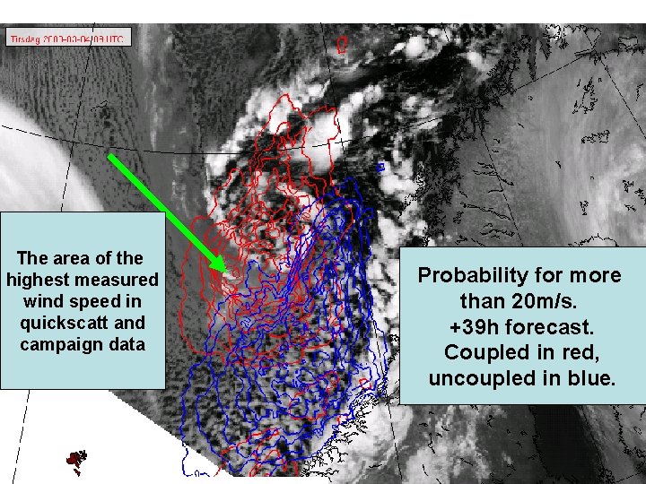
The area of the highest measured wind speed in quickscatt and campaign data Probability for more than 20 m/s. +39 h forecast. Coupled in red, uncoupled in blue.

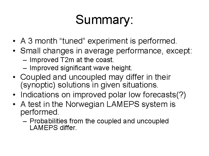
Summary: • A 3 month “tuned” experiment is performed. • Small changes in average performance, except: – Improved T 2 m at the coast. – Improved significant wave height. • Coupled and uncoupled may differ in their (synoptic) solutions in given situations. • Indications on improved polar low forecasts(? ) • A test in the Norwegian LAMEPS system is performed. – Probabilities from the coupled and uncoupled LAMEPS differ.

Surface roughness and fluxes:

The Polar Low 21. January 2007: 03. 22 UTC 21. January 15. 53 UTC 21. January 06. 23 UTC 21. January 01. 31 UTC 22. January

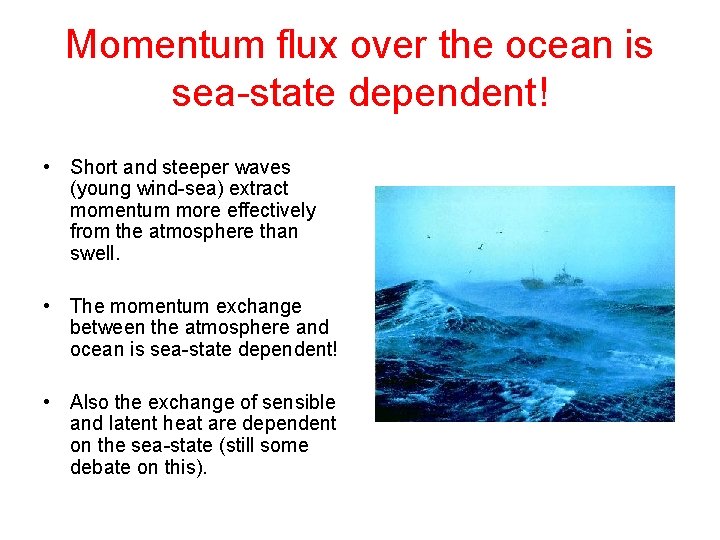
Momentum flux over the ocean is sea-state dependent! • Short and steeper waves (young wind-sea) extract momentum more effectively from the atmosphere than swell. • The momentum exchange between the atmosphere and ocean is sea-state dependent! • Also the exchange of sensible and latent heat are dependent on the sea-state (still some debate on this).

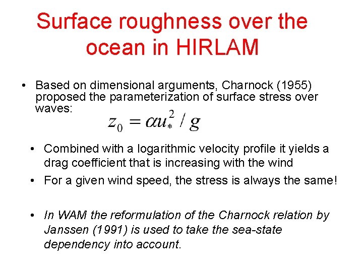
Surface roughness over the ocean in HIRLAM • Based on dimensional arguments, Charnock (1955) proposed the parameterization of surface stress over waves: • Combined with a logarithmic velocity profile it yields a drag coefficient that is increasing with the wind • For a given wind speed, the stress is always the same! • In WAM the reformulation of the Charnock relation by Janssen (1991) is used to take the sea-state dependency into account.

Polar Lows • ”A polar low is a small, but fairly intense maritime cyclone that forms poleward of the main baroclinic zone. The horizontal scale of the polar low is approximately between 200 an 1000 kilometres and surface winds near or above gale force” – Turner, Rasmussen and Carleton in: Polar Lows. Mesoscale Weather systems in the Polar Regions (Ed: Rasmussen and Turner) from 2003 • ”…a polar low is a small-scale synoptic or subsynoptic cyclone that forms in the cold air mass poleward of the main baroclinic zone and/or major secondary frons. It will often be of convective nature but baroclinic effects may be important…” – Rasmussen in Polar and Arctic Lows (Ed: Twitchell, Rasmussen and Davidson) from 1989

Additional comments: • The coupled system show (in average) ~20% higher surface roughness over the ocean. • The coupled system show (in average) 4. 4% higher release of SH from the ocean to the atmosphere. But 1. 4% less release of LH. And in combination the coupled system show (in average) 0. 1% less heat release (LH+SH) from the ocean to the atmosphere. • Coupled and uncoupled are more or less equal in quality on other reported polar lows in the period.

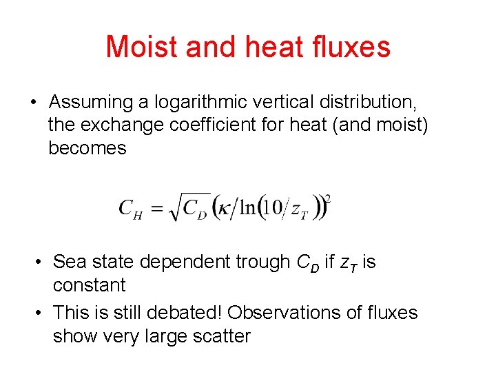
Moist and heat fluxes • Assuming a logarithmic vertical distribution, the exchange coefficient for heat (and moist) becomes • Sea state dependent trough CD if z. T is constant • This is still debated! Observations of fluxes show very large scatter