HighThroughput Sequencing Advanced Microarray Analysis BIOS 691 803

High-Throughput Sequencing Advanced Microarray Analysis BIOS 691 -803, 2008 Dr. Mark Reimers, VCU

Quantitative HTS - Outline • • Technology Preprocessing Quantitative analysis Applications – Ch. IP-Seq – RNA-Seq – Methyl-Seq

The Technology • Most sequencing proceeds by addition of fluor-labeled bases • Do this in parallel on a flat surface • Capture each stage with good camera • Align images

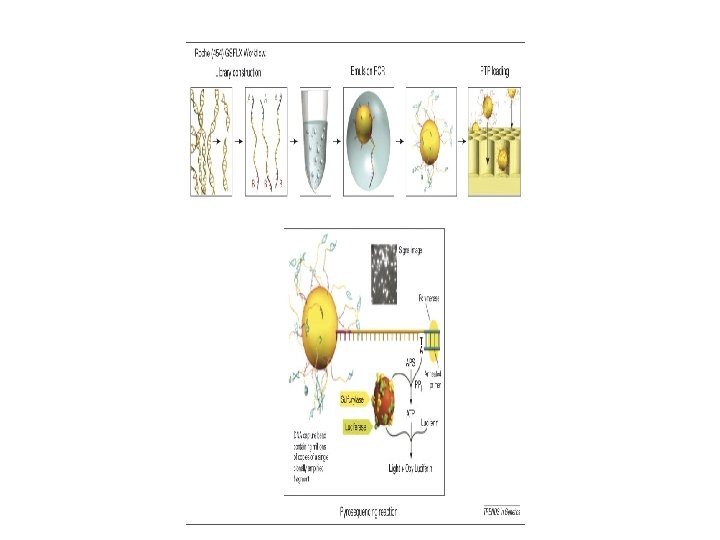
Roche - 454 • Parallel Pyrosequencing on beads

Mardis, Trends in Ge

454 Sequencing Operation

Illumina - Solexa

ABI SOLi. D • Resquencing each fragment with different primers • Reconstruct each fragment separately

Paired-End Reads

Issues • Pre-processing – Base calling – Mapping reads – QA • Quantitative analysis – Variation and noise – Biases – Models – Accuracy and validation

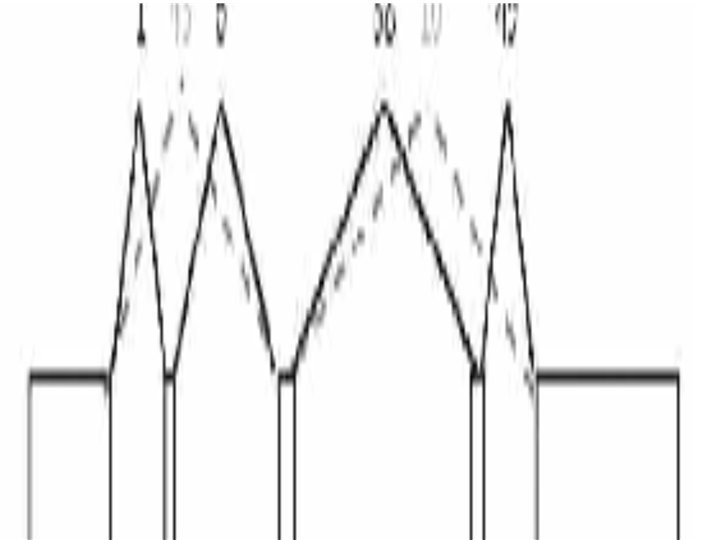
Pre-processing – Base Calling • Not all steps completed properly • Sequence can lag behind or skip ahead • Hence most light spots a mixture of different colors • Simple rule: use brightest signal

Types of mismatches in uniquely mapped tags with a single mismatch are profoundly asymmetric and biased Courtesy Thierry-Mieg

Typical Errors in Base-Calling

Position of single mismatch in uniquely mapped tags Courtesy Thierry-Mieg

Improving Base-Calling with SVM
 BLAT")
Pre-processing – Mapping Reads • • Huge numbers (10 M – 70 M) BLAT (2002 high-speed method) Eland (proprietary Illumina) Other new methods: MAQ, SOAP

Quality Assessment • Fraction of reads mapping to targets • Typically 5 -10 M reads per lane and 60 -80% map to targets • Some repetitive sequence

Comparing Samples - A Simple Normalization • Different numbers of counts per lane • Divide counts in a region of interest (a genomic region or a gene or an exon) by all counts (total per million reads -TPM) • For comparing genomic regions of different lengths divide also by length of region TPKM (total per kilobase per million)

Quant. Analysis - Variation • Poisson model often used for random variation • Most HTS data ‘overdispersed’ relative to Poisson • Negative Binomial often used – Parameter fitted

Quantitative Analysis - Biases • Not all regions represented equally • GC rich regions represented more • Independent of GC some chromosome regions represented more – Euchromatin bias • Sequence initiation site biases • ‘Mapability’ biases – some regions won’t have any uniquely mapped tags

GC Bias • Density of reads depends strongly on GC content of regions GC content (%)

Genomic Position Biases • Count tags from randomly sheared DNA in red with GC content in blue

Start Position Bias

Consistent Start Position Bias Counts per start site in lane 1 vs lane 2

RNA-Seq

RNA-Seq Data Gene Model Kidney Reads Liver Reads From Marioni et al 2008

Accuracy of Illumina RNA-Seq

Comparing RNA-Seq & Affy Issues • How replicable is RNA -Seq? • How consistent are the two technologies? • Which is better? • Marioni et al, Genome Research, 2008

Comparing Fold-Changes • D. E. by ILM • Red >250 • Green <250 • Black Not DE by ILM

Model for Variation • Poisson counts hypergeometric comparison • Make uniform p-values by adding random term – Use lower tails only

False Positive Rates • QQ-plots of p-values between tech. reps

Different Concentrations are NOT Comparable! • QQ-plots of p-values between 3 p. M and 1. 5 p. M

Normalization of RNA-Seq • Robinson et al noticed that most genes appeared less expressed in liver Fig 1 from Robinson & Oshlak, Genome Biology 2010

A Better Normalization for RNASeq - TMM • • Drop extremes of ratios Drop very high count genes Compute trimmed means of samples Center log-ratios between samples

New Things to do with RNA-Seq • Allele-specific expression • Splice variation – Between tissues – In disease • Alternate initiation sites – Select 5’ capped RNA fragments • Alternate termination

Allelic Comparison • It is possible to compare allele-specific expression counts • Sample from VCU • Replicate samples • P-values for binomial tests of equality • About half show differential expression!

Detecting Splice Variation • Deep sequencing shows up clear variation in exon usage • Wang et al Nature 2008

Tissue Map of Splice Variation From Wang et al • Brain is most distinctive • Individuals seem to differ • Cell lines seem to have distinct splice patterns

Splicing is Complex • Many different splice operations exist • Only some of these characterized by counting exon reads
")
Issues in Detecting Splice Variants • Counts in exons reflect biases (as yet uncharacterized) as well as actual abundance • Reads that bridge splice junctions would be definitive but mapping is very dubious with short (<40 base) reads • All possible splice junctions are not known – Hard to even search through the known ones

Methodology for Splice Variants • Count reads mapped to exons and compare ratios across samples – Wang et al, and most others • Count reads that cross splice junctions

Methodology for Finding Junctions

Ch. IP-Seq

Chromatin Immuno-precipitation

Ch. IP-Seq Workflow • • • Cross-link proteins to DNA Fragment DNA Extract with antibody Reverse cross links Sequence fragments DO CONTROLS!

Ch. IP-Seq Data • From Rozowsky et al, Nature Biotech 2009

Ch. IP-Seq vs Ch. IP-chip

Peak-Finding - Simple • Extend tags and count overlap • How much to extend?

Peak Finding – Better • Tags starting on opposite strands are likely to start at opposite ends • Identifying the cross-over point leads to improved accuracy

The Value of Controls: Ch. IP vs. Control Reads Red dots are windows containing Ch. IP peaks and black dots are windows containing control peaks used for FDR calculation

Cause of Variation in Read Density • In study of Fox. A 1 binding, even control reads enriched near Fox. A 1 binding site! • Probably due to open chromatin near Fox. A 1 binding site Density of Control Channel reads around Fox. A 1 site Courtesy Shirley Liu

Ch. IP-Seq – MACS Key Ideas • Smart peak imputation estimate – Uses read directions – Empirical estimate of fragment length • Local frequency estimate – Using control, if available – Using wide estimate, otherwise – Not using sequence

Read Lengths and Directions • Some clear clusters – even before stats • Reads on opposite sides of peak map to opposite strands – Hence fragments have opposite directions • Can estimate apparent fragment length

Fragment Lengths • Puzzle: Fragments from sonication expected to be between 200 – 500 bp • Estimated fragment size ~ 100 bp • Shirley Liu’s explanation: preferential cutting near to TF ? ?

Comparison to Ch. IP-chip • Broad correlation • Not dramatic improvement in precision !

Methyl-Seq
 • Methylation-specific")
Methylation Assays • Affinity purification: e. g. Me. DIP-Seq (methylated dinucleotide immunoprecipitation) • Methylation-specific cleavage by endonucleases – e. g. Methyl-Seq: Cleaves with HPA 2 to identify • Bisulphite conversion – WGBS (Whole-Genome Bisulphite Sequencing) – RRBS (Reduced Representation Bisulphite Sequencing) • Cleaves with MSPI to reduce complexity

Affinity: Me. DIP-Seq & MBD-Seq

Issues with Affinity Methods • Analysis essentially like Ch. IP-Seq • BUT: Sequence count reflects both density of Cp. G’s and proportions of methylation • No individual Cp. G-level information • Advantages: no conversion so sequence tags are easily mappable

Methyl-Seq • Use HPAII to cleave only at unmethylated CCGG sites • Size-select fragments (50 -300) • Sequence fragment ends – Always starting at a CCGG • Easy to map – few possible loci (<1 M) • Paired ends give actual fragment

Schematic Here

Issues for Methyl Seq • Computational problem to re-assemble actual proportions of methylation at each locus from counts • Prone to false positives because of incomplete digestion (for reasons other than methylation of CCGG site) – e. g. insufficient time … – rates vary by 50 -fold depending on sequence context

WGBS • Bisulphite conversion, fragmentation and shotgun sequencing • Requires very many reads! • Use of capture arrays reduces work… BUT different sequences have different capture efficiencies!
 • top, CHP-SKN-1; bottom, MDA-MB-231 • NB. Inconsistent tag")
WGBS Data (from capture array) • top, CHP-SKN-1; bottom, MDA-MB-231 • NB. Inconsistent tag numbers

Issues with WGBS • Lose many C’s • Hard to map to genome • Strategy depends on less penalty for mapping T to C • Too many loci!

RRBS • Too many methylation sites in genome • Cleave with MSPI and size select in order to reduce number of fragments • Convert C to T with bisulphite (not m. C) • Then sequence fragments • 1. 4 M fragments

Issues with RRBS • Fairly broad but not complete coverage of ‘interesting’ regions of genome • Bisulphite conversion of limited regions means mapping is fairly easy • Bisulphite conversion not always complete

Meta-Genomics

What is Meta-genomics? • Sequencing random fragments of DNA from all microbial denizens of a community (and traces of a few others) • Sometimes broadly used for surveys of microbial diversity based on sequencing all 16 Sr. RNA genes present

Kinds of Questions • What is out there? – Most microbial species not known • What metabolic fluxes in any environment? • What microbes associated with specific conditions? – Including disease or health • Human Microbiome Project

Environmental Meta-Genomics

Human Microbiome Project

Data Analysis Issues – 16 S r. RNA • Identification of microbes – most are unknown and un-culturable • Distinguishing errors in sequencing from novel microbes • Biases in sequencing

Data Analysis Issues - Metagenomics • Mapping and characterizing unknown protein sequences • Usually assume conservation • Full-coverage allows assembly of genomes • Counting • Biases probably smaller (Bork)
- Slides: 76