Highrate drift chamber hit reconstruction with machine learning

機械学習を活用した 高計数率ドリフトチェンバー のヒット再構成 High-rate drift chamber hit reconstruction with machine learning technique 内山 雄祐 (The University of Tokyo) on behalf of MEG II collaboration 日本物理学会 2021年年次大会 令和3年 3月14日 14 a. T 3 -7

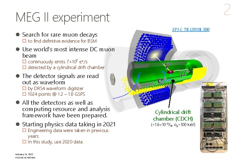
2 MEG II experiment EPJ-C 78 (2018) 380 l Search for rare muon decays p to find definitive evidence for BSM l Use world’s most intense DC muon beam p continuously emits 7× 107 e+/s p detected by a cylindrical drift chamber l The detector signals are read out as waveform p by DRS 4 waveform digitizer p 1024 points @ 1. 2 – 1. 8 GSPS l All the detectors as well as computing resource and analysis framework have been prepared. l Starting physics data taking in 2021 p Engineering data were taken in previous years. p In this study, use 2020 data. February 14, 2022 YUSUKE UCHIYAMA γ e+ μ+ Cylindrical drift chamber (CDCH) (~1. 6× 10 -3 X 0, σp~100 ke. V)

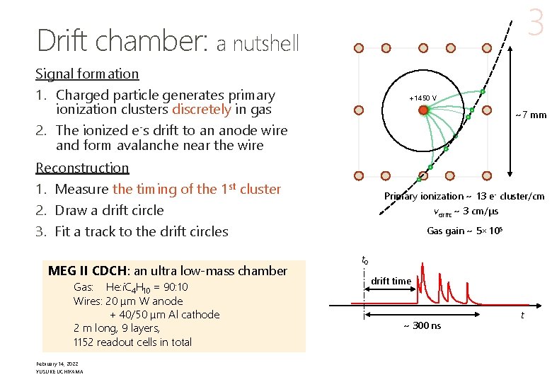
3 Drift chamber: a nutshell Signal formation 1. Charged particle generates primary ionization clusters discretely in gas 2. The ionized e-s drift to an anode wire and form avalanche near the wire +1450 V ~7 mm Reconstruction 1. Measure the timing of the 1 st cluster 2. Draw a drift circle 3. Fit a track to the drift circles MEG II CDCH: an ultra low-mass chamber Gas: He: i. C 4 H 10 = 90: 10 Wires: 20 μm W anode + 40/50 μm Al cathode 2 m long, 9 layers, 1152 readout cells in total February 14, 2022 YUSUKE UCHIYAMA Primary ionization ~ 13 e- cluster/cm vdrift ~ 3 cm/μs Gas gain ~ 5× 105 t 0 drift time ~ 300 ns t

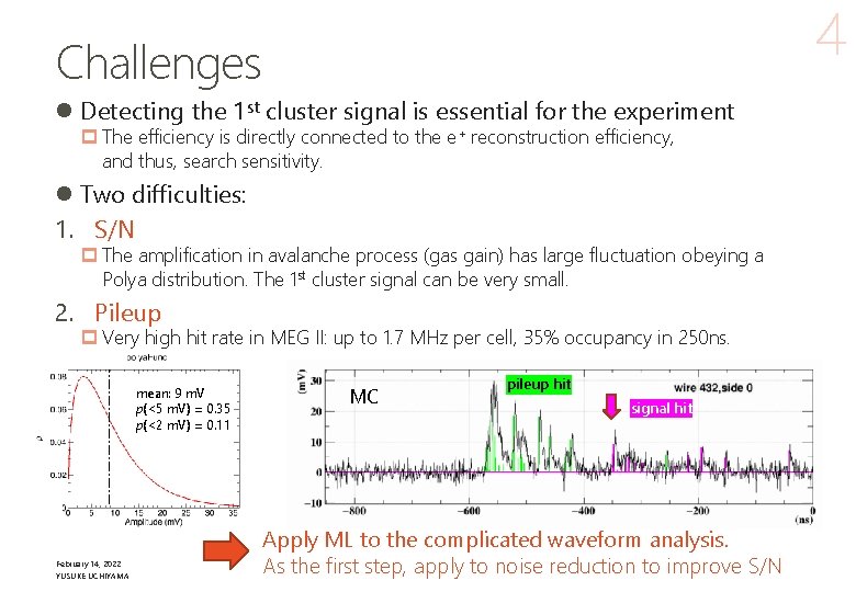
4 Challenges l Detecting the 1 st cluster signal is essential for the experiment p The efficiency is directly connected to the e+ reconstruction efficiency, and thus, search sensitivity. l Two difficulties: 1. S/N p The amplification in avalanche process (gas gain) has large fluctuation obeying a Polya distribution. The 1 st cluster signal can be very small. 2. Pileup p Very high hit rate in MEG II: up to 1. 7 MHz per cell, 35% occupancy in 250 ns. mean: 9 m. V p(<5 m. V) = 0. 35 p(<2 m. V) = 0. 11 February 14, 2022 YUSUKE UCHIYAMA MC pileup hit signal hit Apply ML to the complicated waveform analysis. As the first step, apply to noise reduction to improve S/N

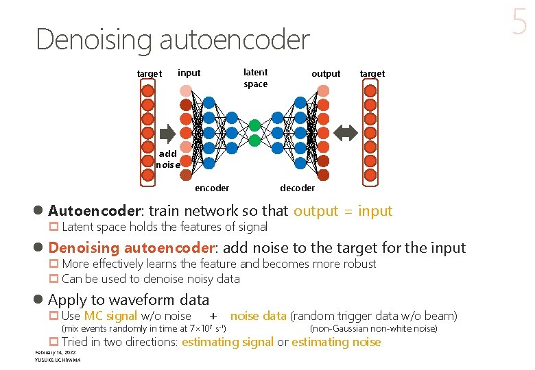
5 Denoising autoencoder target latent space input output target add noise encoder decoder l Autoencoder: train network so that output = input p Latent space holds the features of signal l Denoising autoencoder: add noise to the target for the input p More effectively learns the feature and becomes more robust p Can be used to denoise noisy data l Apply to waveform data p Use MC signal w/o noise + (mix events randomly in time at 7× 107 s-1) noise data (random trigger data w/o beam) (non-Gaussian non-white noise) p Tried in two directions: estimating signal or estimating noise February 14, 2022 YUSUKE UCHIYAMA

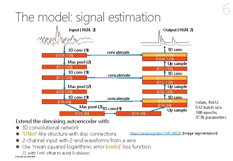
6 The model: signal estimation Input (1024, 2) 1 D conv (9) (1024, 128) Output (1024, 2) 1 D conv concatenate (1024, 128) Max pool (2) Up sample (512, 128) 1 D conv (9) (512, 128) 1 D conv concatenate (512, 128) Max pool (2) Up sample (256, 128) 1 D conv (9) (256, 64) Max pool (2)1 D conv(9) (128, 64) 1 D conv concatenate (256, 64) (128, 64) Up sample Adam, Re. LU, 512 batch size, 100 epochs, 373 k parameters Extend the denoising autoencoder with: l 1 D convolutional network https: //arxiv. org/abs/1505. 04597 (image segmentation) l ‘UNet’-like structure with skip connections l 2 -channel input with 2 -end waveforms from a wire l Use ‘mean squared logarithmic error (msle)’ loss function. p with 1 m. V offset to avoid 0 -division. February 14, 2022 YUSUKE UCHIYAMA

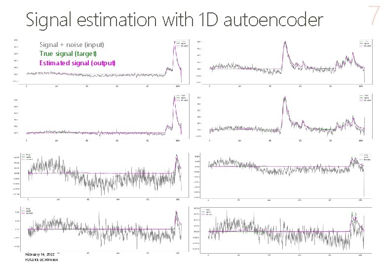
Signal estimation with 1 D autoencoder Signal + noise (input) True signal (target) Estimated signal (output) February 14, 2022 YUSUKE UCHIYAMA 7

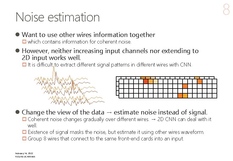
Noise estimation l Want to use other wires information together p which contains information for coherent noise. l However, neither increasing input channels nor extending to 2 D input works well. p It is difficult to extract different signal patterns in different wires with CNN. l Change the view of the data → estimate noise instead of signal. p Coherent noise changes gradually over different wires. → 2 D CNN can deal with it well. p Existence of signal masks the noise, but estimate it using other wires waveform. p Group 8 wires that connect to the same front-end cards into an input. February 14, 2022 YUSUKE UCHIYAMA 8

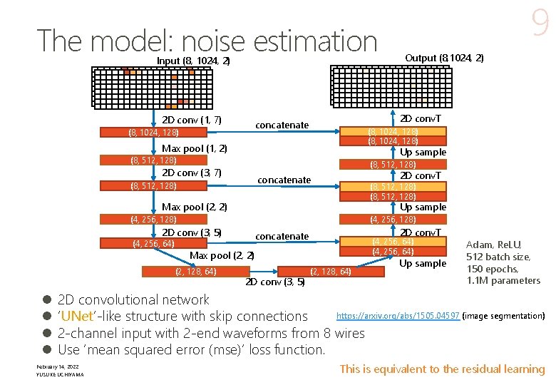
The model: noise estimation Input (8, 1024, 2) 2 D conv (1, 7) (8, 1024, 128) Max pool (1, 2) Up sample (8, 512, 128) 2 D conv (3, 7) 2 D conv. T concatenate (8, 512, 128) Max pool (2, 2) Up sample (4, 256, 128) 2 D conv (3, 5) (4, 256, 64) 2 D conv. T concatenate (4, 256, 64) Max pool (2, 2) (2, 128, 64) l l Output (8, 1024, 2) 2 D conv. T concatenate (8, 1024, 128) 9 2 D conv (3, 5) (2, 128, 64) Up sample Adam, Re. LU, 512 batch size, 150 epochs, 1. 1 M parameters 2 D convolutional network https: //arxiv. org/abs/1505. 04597 (image segmentation) ‘UNet’-like structure with skip connections 2 -channel input with 2 -end waveforms from 8 wires Use ‘mean squared error (mse)’ loss function. February 14, 2022 YUSUKE UCHIYAMA This is equivalent to the residual learning

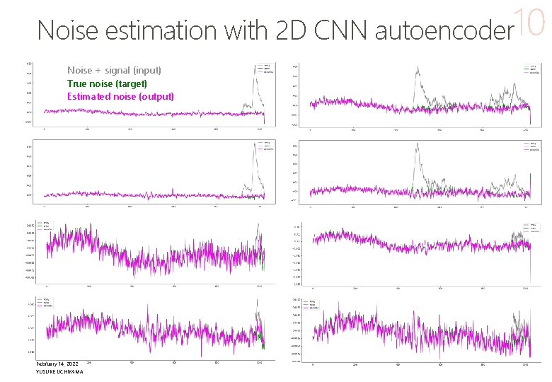
Noise estimation with 2 D CNN autoencoder 10 Noise + signal (input) True noise (target) Estimated noise (output) February 14, 2022 YUSUKE UCHIYAMA

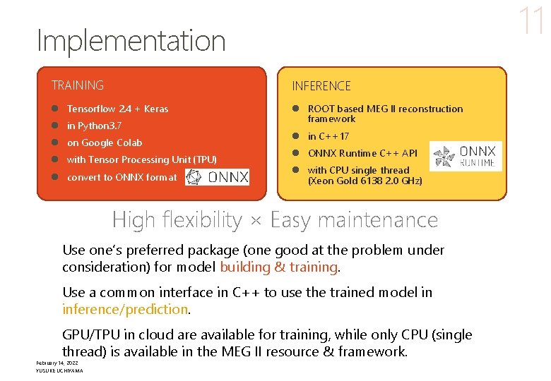
11 Implementation TRAINING INFERENCE l Tensorflow 2. 4 + Keras l ROOT based MEG II reconstruction framework l in Python 3. 7 l on Google Colab l with Tensor Processing Unit (TPU) l convert to ONNX format l in C++17 l ONNX Runtime C++ API l with CPU single thread (Xeon Gold 6138 2. 0 GHz) High flexibility × Easy maintenance Use one’s preferred package (one good at the problem under consideration) for model building & training. Use a common interface in C++ to use the trained model in inference/prediction. GPU/TPU in cloud are available for training, while only CPU (single thread) is available in the MEG II resource & framework. February 14, 2022 YUSUKE UCHIYAMA

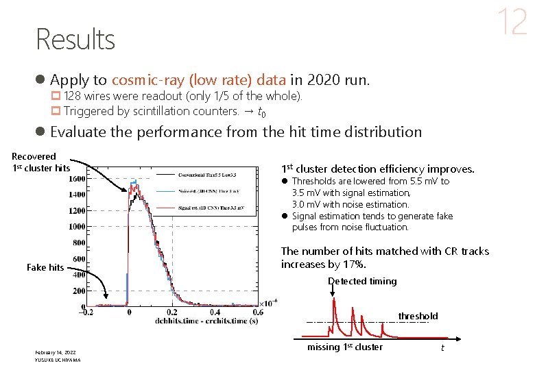
12 Results l Apply to cosmic-ray (low rate) data in 2020 run. p 128 wires were readout (only 1/5 of the whole). p Triggered by scintillation counters. → t 0 l Evaluate the performance from the hit time distribution Recovered 1 st cluster hits 1 st cluster detection efficiency improves. l Thresholds are lowered from 5. 5 m. V to 3. 5 m. V with signal estimation, 3. 0 m. V with noise estimation. l Signal estimation tends to generate fake pulses from noise fluctuation. Fake hits The number of hits matched with CR tracks increases by 17%. Detected timing threshold February 14, 2022 YUSUKE UCHIYAMA missing 1 st cluster t

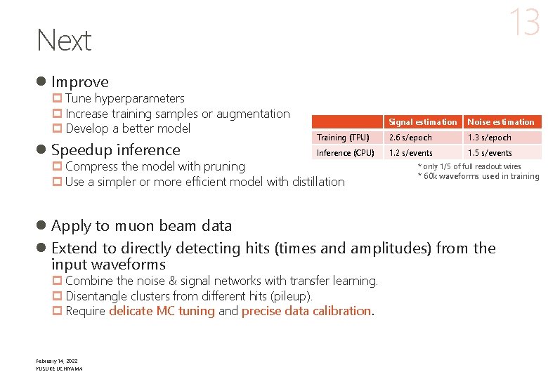
13 Next l Improve p Tune hyperparameters p Increase training samples or augmentation p Develop a better model l Speedup inference Signal estimation Noise estimation Training (TPU) 2. 6 s/epoch 1. 3 s/epoch Inference (CPU) 1. 2 s/events 1. 5 s/events p Compress the model with pruning p Use a simpler or more efficient model with distillation * only 1/5 of full readout wires * 60 k waveforms used in training l Apply to muon beam data l Extend to directly detecting hits (times and amplitudes) from the input waveforms p Combine the noise & signal networks with transfer learning. p Disentangle clusters from different hits (pileup). p Require delicate MC tuning and precise data calibration. February 14, 2022 YUSUKE UCHIYAMA

Conclusions l Applied denoising autoencoders to MEG II CDCH waveform data. l The models certainly learn the features of signal and noise. l Denoising enables lowering hit detection threshold and improves the detection efficiency of the 1 st cluster signal. p Superior to conventional waveform analysis with digital filters. p A promising technique to improve the experiment sensitivity. l Flexible & sustainable framework matching HEP analysis was established. l Computation time in inference is an issue for practical application, p in which only single thread CPU is available. p Speeding up by a factor 5 is desirable. February 14, 2022 YUSUKE UCHIYAMA 14

15 l 1 D conv ⇔ FIR digital filter. Apply multiple filters to catch different patterns. l Activation → nonlinear response. l CNN → position invariant signal detection, but not scale invariant → learn from data. ←Augmentation will help it. l Pooling → allow timing variation, good for local pattern recognition but loose global timing information l U-net skip connection → recover global timing information February 14, 2022 YUSUKE UCHIYAMA

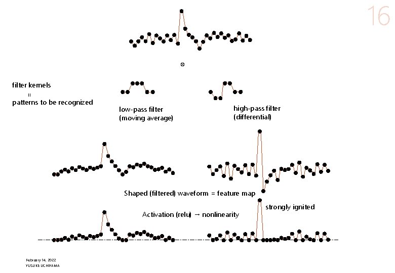
16 ⊗ filter kernels = patterns to be recognized low-pass filter (moving average) high-pass filter (differential) Shaped (filtered) waveform = feature map Activation (relu) → nonlinearity February 14, 2022 YUSUKE UCHIYAMA strongly ignited

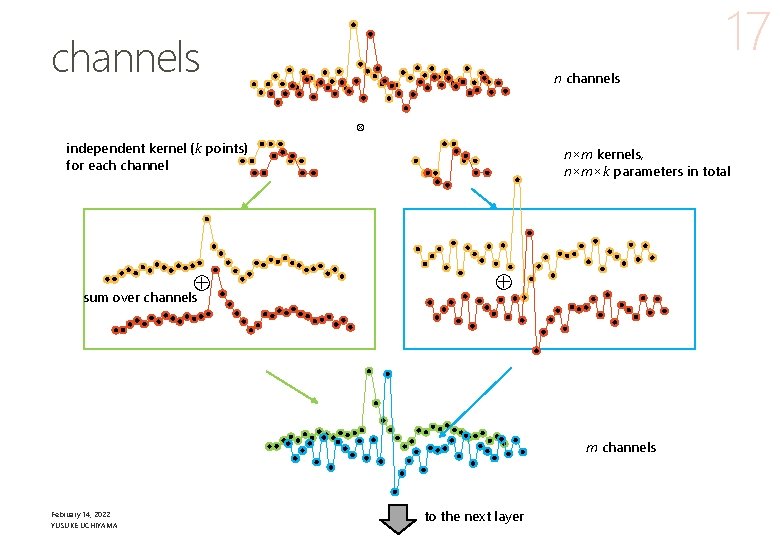
17 channels n channels ⊗ independent kernel (k points) for each channel ⊕ sum over channels n×m kernels, n×m×k parameters in total ⊕ m channels February 14, 2022 YUSUKE UCHIYAMA to the next layer

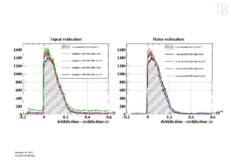
18 Signal estimation February 14, 2022 YUSUKE UCHIYAMA Noise estimation

19 ONNX l The best solution as of today, we concluded, is using ONNX. l Open Neural Network Exchange (ONNX) is an open standard format for representing machine learning models. p Able to exchange the models built by different frameworks. Supported by February 14, 2022 YUSUKE UCHIYAMA

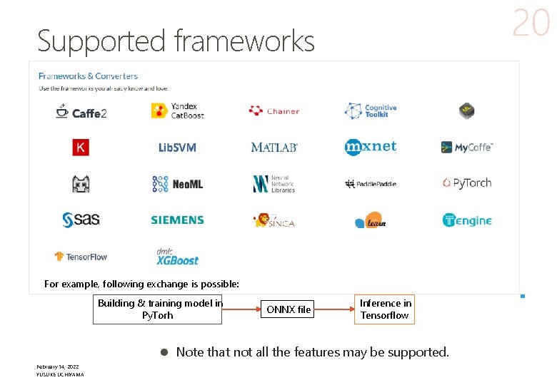
20 Supported frameworks For example, following exchange is possible: Building & training model in Py. Torh ONNX file Inference in Tensorflow l Note that not all the features may be supported. February 14, 2022 YUSUKE UCHIYAMA

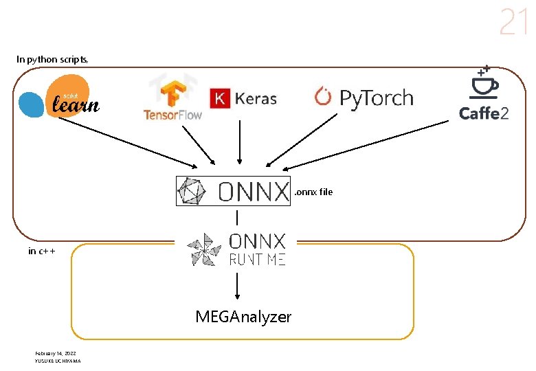
21 In python scripts, . onnx file in c++ MEGAnalyzer February 14, 2022 YUSUKE UCHIYAMA

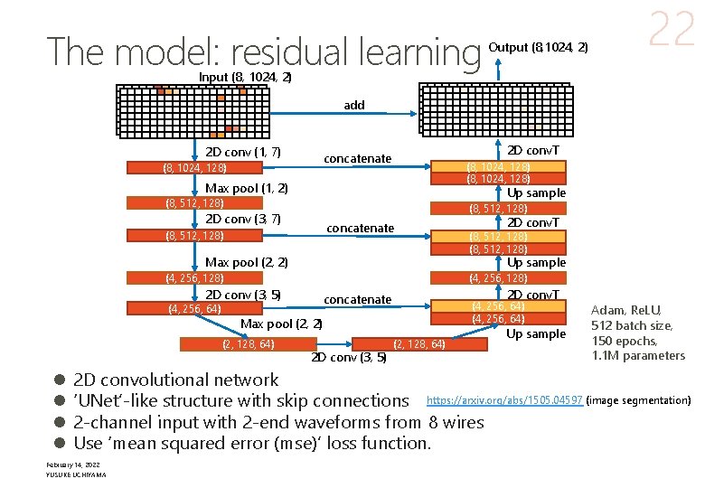
The model: residual learning Output (8, 1024, 2) 22 Input (8, 1024, 2) add 2 D conv (1, 7) 2 D conv. T concatenate (8, 1024, 128) Max pool (1, 2) Up sample (8, 512, 128) 2 D conv (3, 7) concatenate (8, 512, 128) Max pool (2, 2) (4, 256, 128) 2 D conv (3, 5) 2 D conv. T concatenate (4, 256, 64) Max pool (2, 2) (2, 128, 64) l l (8, 512, 128) Up sample (4, 256, 128) (4, 256, 64) 2 D conv. T 2 D conv (3, 5) (2, 128, 64) Up sample Adam, Re. LU, 512 batch size, 150 epochs, 1. 1 M parameters 2 D convolutional network ‘UNet’-like structure with skip connections https: //arxiv. org/abs/1505. 04597 (image segmentation) 2 -channel input with 2 -end waveforms from 8 wires Use ‘mean squared error (mse)’ loss function. February 14, 2022 YUSUKE UCHIYAMA