Highdimensional integration without Markov chains Alexander Gray Carnegie

High-dimensional integration without Markov chains Alexander Gray Carnegie Mellon University School of Computer Science

High-dimensional integration by: • Nonparametric statistics • Computational geometry • Computational physics • Monte Carlo methods • Machine learning • . . . …but NOT Markov chains.

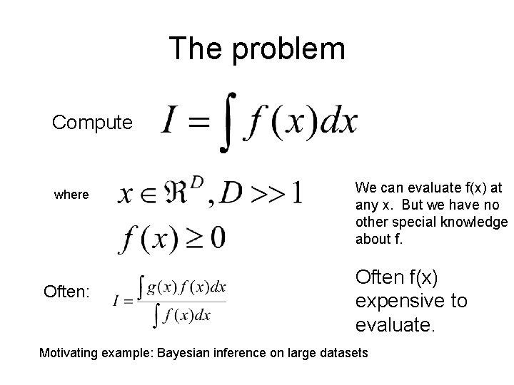
The problem Compute where Often: We can evaluate f(x) at any x. But we have no other special knowledge about f. Often f(x) expensive to evaluate. Motivating example: Bayesian inference on large datasets

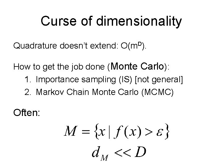
Curse of dimensionality Quadrature doesn’t extend: O(m. D). How to get the job done (Monte Carlo): 1. Importance sampling (IS) [not general] 2. Markov Chain Monte Carlo (MCMC) Often:

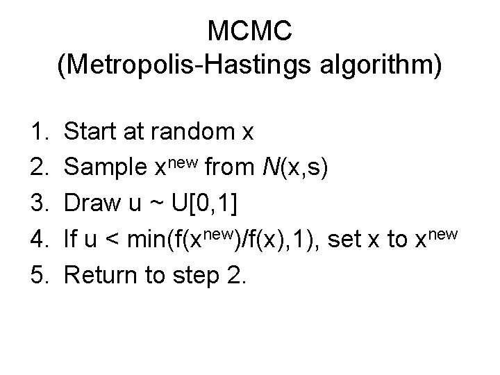
MCMC (Metropolis-Hastings algorithm) 1. 2. 3. 4. 5. Start at random x Sample xnew from N(x, s) Draw u ~ U[0, 1] If u < min(f(xnew)/f(x), 1), set x to xnew Return to step 2.

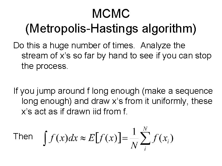
MCMC (Metropolis-Hastings algorithm) Do this a huge number of times. Analyze the stream of x’s so far by hand to see if you can stop the process. If you jump around f long enough (make a sequence long enough) and draw x’s from it uniformly, these x’s act as if drawn iid from f. Then

Good Really cool: – Ultra-simple – Requires only evaluations of f – Faster than quadrature in high dimensions gave us the bomb (? ? ) listed in “Top 10 algorithms of all time”

Bad Really unfortunate: 1. No reliable way to choose the scale s; yet, its choice is critical for good performance 2. With multiple modes, can get stuck 3. Correlated sampling is hard to characterize in terms of error 4. Prior knowledge can be incorporated only in simple ways 5. No way to reliably stop automatically Requires lots of runs/tuning/guesswork. Many workarounds, for different knowledge about f. (Note that in general case, almost nothing has changed. ) Must become an MCMC expert just to do integrals. (…and the ugly) In the end, we can’t be quite sure about our answer. Black art. Not yet in Numerical Recipes.

Let’s try to make a new method Goal: – Simple like MCMC – Weak/no requirements on f() – Principled and automatic choice of key parameter(s) – Real error bounds – Better handling of isolated modes – Better incorporation of prior knowledge – Holy grail: automatic stopping rule

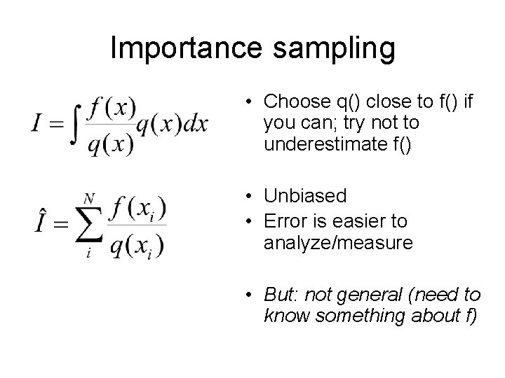
Importance sampling • Choose q() close to f() if you can; try not to underestimate f() • Unbiased • Error is easier to analyze/measure • But: not general (need to know something about f)

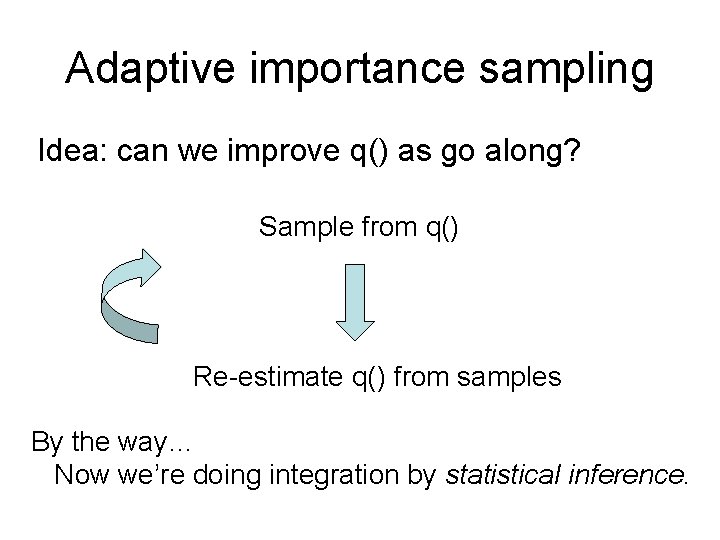
Adaptive importance sampling Idea: can we improve q() as go along? Sample from q() Re-estimate q() from samples By the way… Now we’re doing integration by statistical inference.

NAIS [Zhang, JASA 1996] Assume f() is a density. 1. Generate x’s from an initial q() 2. Estimate density fhat from the x’s, using kernel density estimation (KDE): 3. Sample x’s from fhat. 4. Return to step 2.

Some attempts for q() • Kernel density estimation [e. g. Zhang, JASA 1996] – O(N 2); choice of bandwidth • Gaussian process regression [e. g. Rasmussen. Ghahramani, NIPS 2002] – O(N 3); choice of bandwidth • Mixtures (of Gaussians, betas…) [e. g. Owen-Zhou 1998] – nonlinear unconstrained optimization is itself time-consuming and contributes variance; choice of k, … • Neural networks [e. g. JSM 2003] – (let’s get serious) awkward to sample from; like mixtures but worse Bayesian quadrature: right idea but not general

None of these works (i. e. is a viable alternative to MCMC)

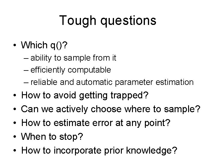
Tough questions • Which q()? – ability to sample from it – efficiently computable – reliable and automatic parameter estimation • • • How to avoid getting trapped? Can we actively choose where to sample? How to estimate error at any point? When to stop? How to incorporate prior knowledge?

What’s the right thing to do? (i. e. what objective function should we be optimizing? )

Is this active learning (aka optimal experiment design)? Basic framework: bias-variance decomposition of leastsquares objective function minimize only variance term Seems reasonable, but: • Is least-squares really the optimal thing to do for our problem (integration)?

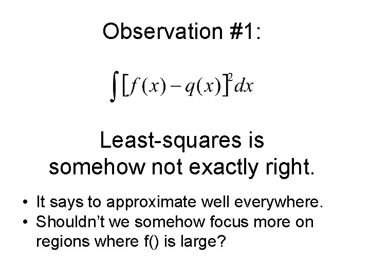
Observation #1: Least-squares is somehow not exactly right. • It says to approximate well everywhere. • Shouldn’t we somehow focus more on regions where f() is large?

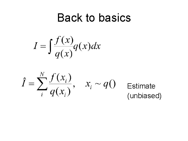
Back to basics Estimate (unbiased)

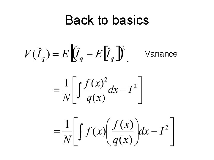
Back to basics Variance

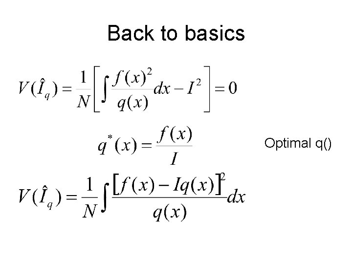
Back to basics Optimal q()

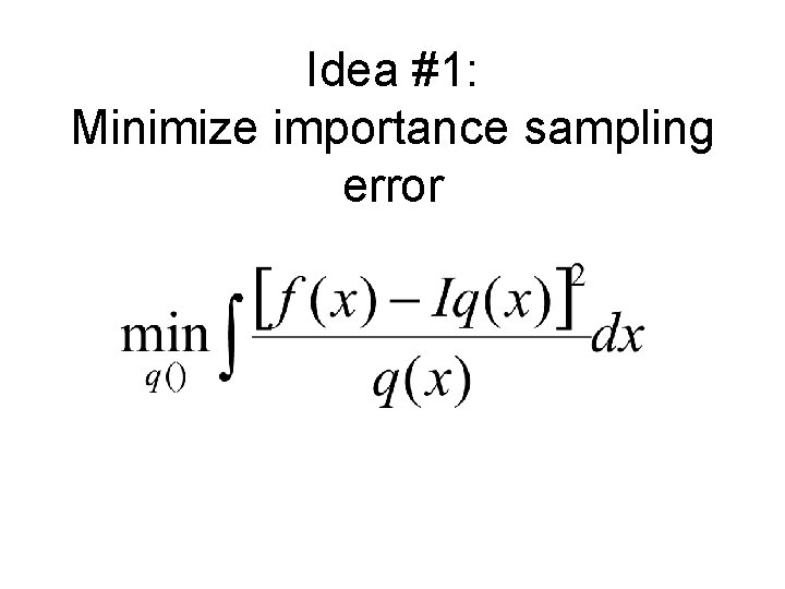
Idea #1: Minimize importance sampling error

Error estimate cf. [Neal 1996]: Use - indirect and approximate argument - can use for stopping rule

What kind of estimation?

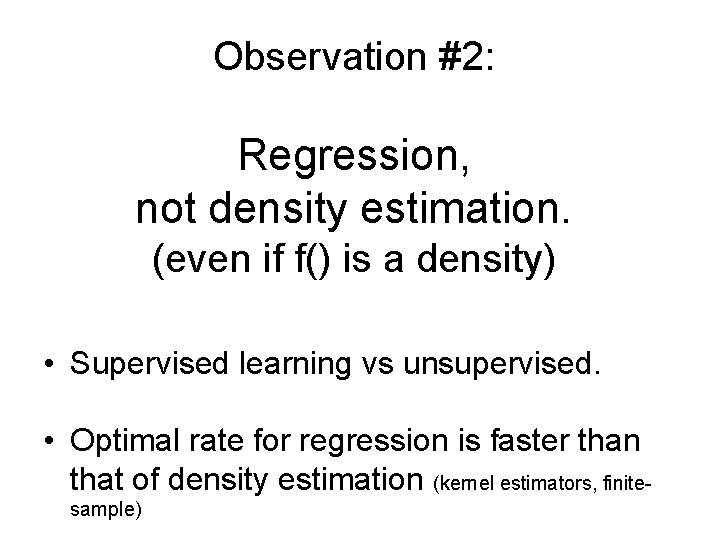
Observation #2: Regression, not density estimation. (even if f() is a density) • Supervised learning vs unsupervised. • Optimal rate for regression is faster than that of density estimation (kernel estimators, finitesample)

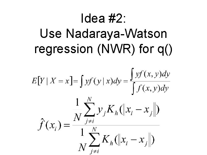
Idea #2: Use Nadaraya-Watson regression (NWR) for q()

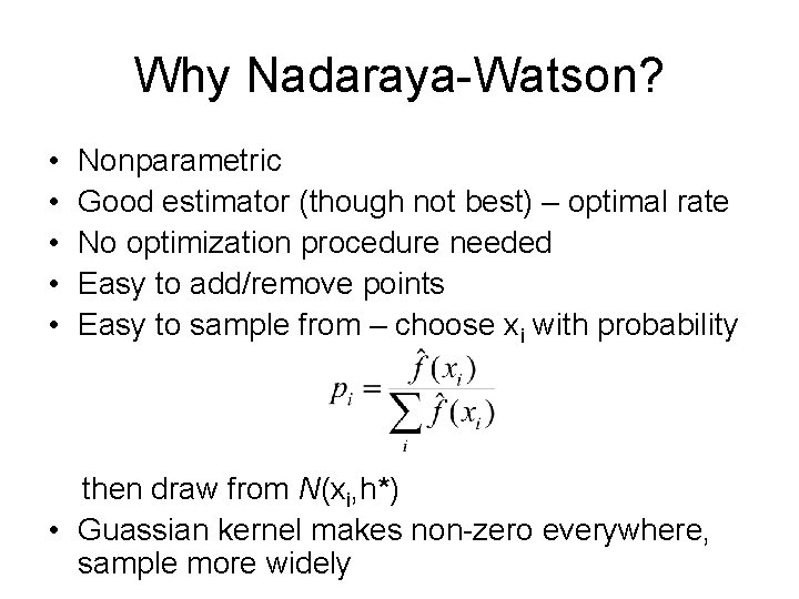
Why Nadaraya-Watson? • • • Nonparametric Good estimator (though not best) – optimal rate No optimization procedure needed Easy to add/remove points Easy to sample from – choose xi with probability then draw from N(xi, h*) • Guassian kernel makes non-zero everywhere, sample more widely

How can we avoid getting trapped?

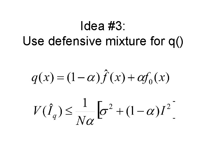
Idea #3: Use defensive mixture for q()

This also answered: “How can we incorporate prior knowledge”?

Can we do NWR tractably?

Observation #3: NWR is a ‘generalized N-body problem’. • distances between n-tuples [pairs] of points in a metric space [Euclidean] • modulated by a (symmetric) positive monotonic kernel [pdf] • decomposable operator [summation]

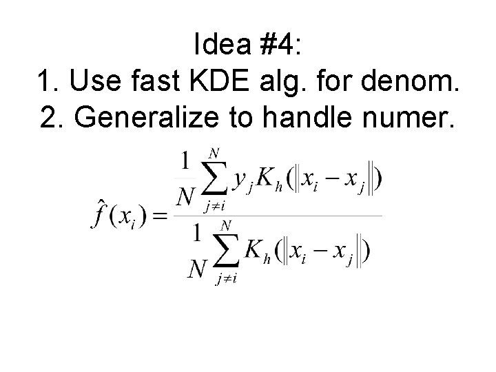
Idea #4: 1. Use fast KDE alg. for denom. 2. Generalize to handle numer.

Extension from KDE to NWR • First: allow weights on each point • Second: allow those weights to be negative • Not hard

Okay, so we can compute NWR efficiently with accuracy. How do we find the bandwidth (accurately and efficiently)?

What about an analytical method? Bias-variance decomposition has many terms that can be estimated (if very roughly) But the real problem is D. Thus, this is not reliable in our setting.

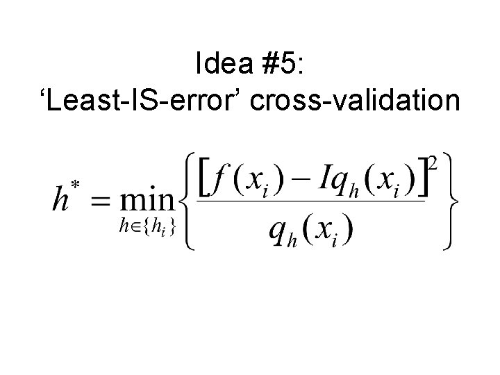
Idea #5: ‘Least-IS-error’ cross-validation

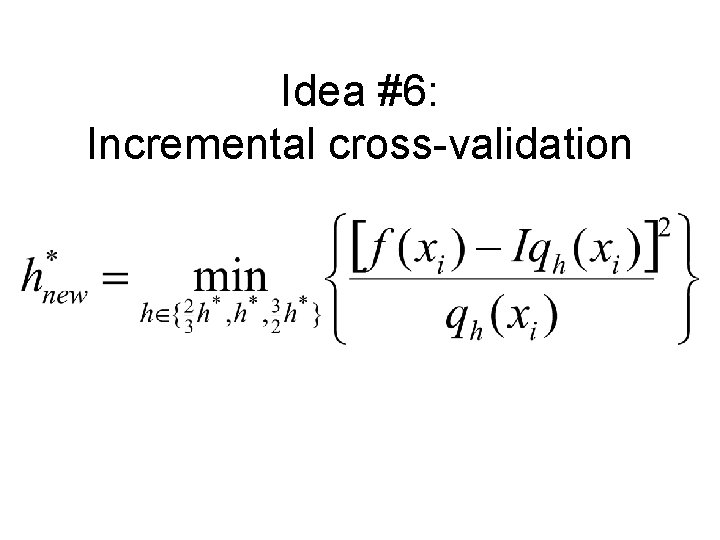
Idea #6: Incremental cross-validation

Idea #7: Simultaneous-bandwidth N-body algorithm We can share work between bandwidths. [Gray and Moore, 2003]

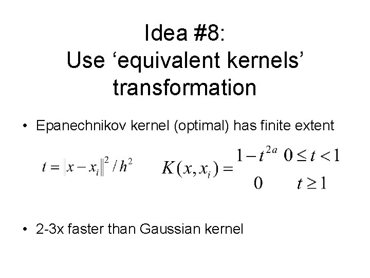
Idea #8: Use ‘equivalent kernels’ transformation • Epanechnikov kernel (optimal) has finite extent • 2 -3 x faster than Gaussian kernel

How can we pick samples in a guided fashion? • Go where we’re uncertain? • Go by the f() value, to ensure low intrinsic dimension for the N-body algorithm?

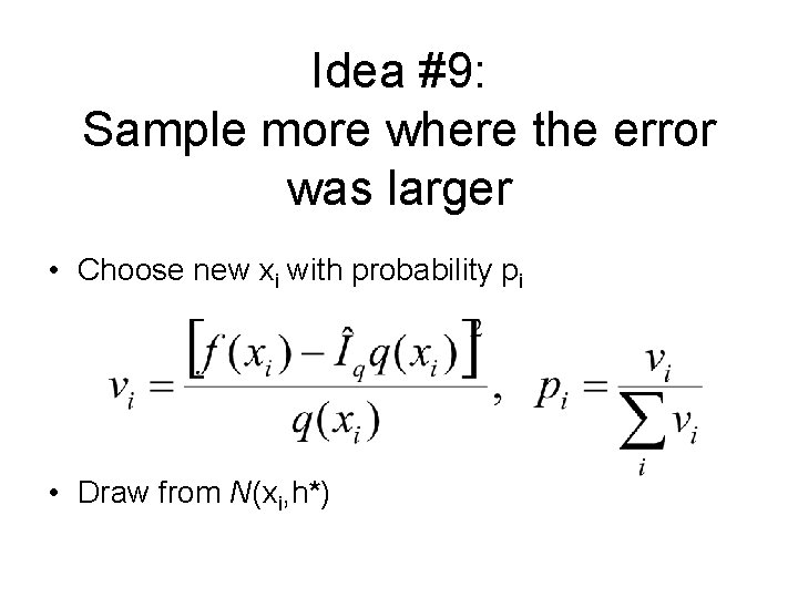
Idea #9: Sample more where the error was larger • Choose new xi with probability pi • Draw from N(xi, h*)

Should we forget old points? I tried that. It doesn’t work. So I remember all the old samples.

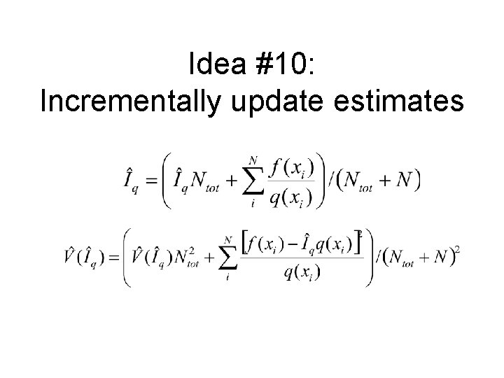
Idea #10: Incrementally update estimates

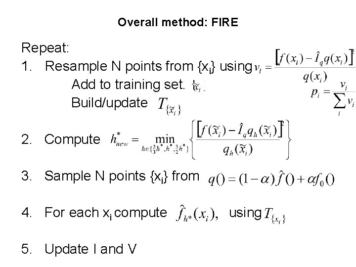
Overall method: FIRE Repeat: 1. Resample N points from {xi} using Add to training set. Build/update 2. Compute 3. Sample N points {xi} from 4. For each xi compute 5. Update I and V using

Properties • Because FIRE is importance sampling: – consistent – unbiased • The NWR estimate approaches f(x)/I • Somewhat reminiscent of particle filtering; EM-like; like N interacting Metropolis samplers

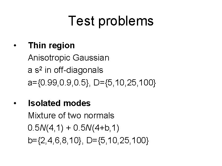
Test problems • Thin region Anisotropic Gaussian a s 2 in off-diagonals a={0. 99, 0. 5}, D={5, 10, 25, 100} • Isolated modes Mixture of two normals 0. 5 N(4, 1) + 0. 5 N(4+b, 1) b={2, 4, 6, 8, 10}, D={5, 10, 25, 100}

Competitors • Standard Monte Carlo • MCMC (Metropolis-Hastings) – starting point [Gelman-Roberts-Gilks 95] – adaptation phase [Gelman-Roberts-Gilks 95] – burn-in time [Geyer 92] – multiple chains [Geyer 92] – thinning [Gelman 95]

How to compare Look at its relative error over many runs When to stop it? 1. Use its actual stopping criterion 2. Use a fixed wall-clock time

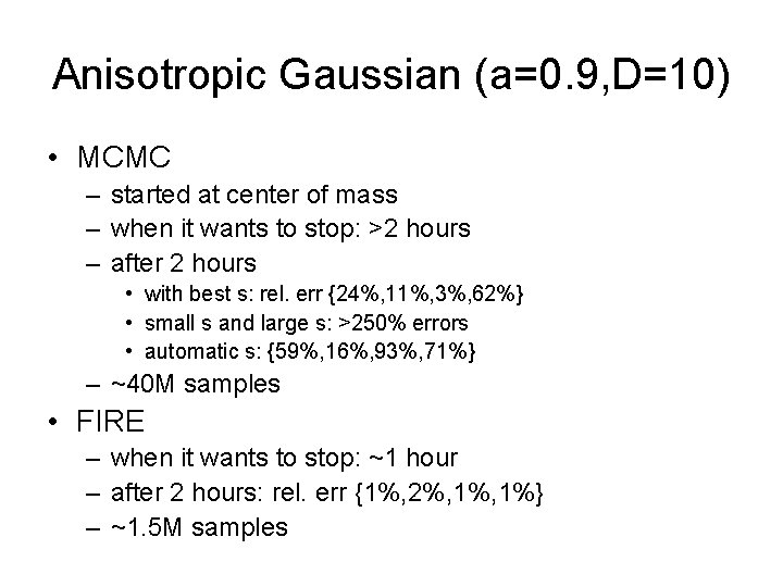
Anisotropic Gaussian (a=0. 9, D=10) • MCMC – started at center of mass – when it wants to stop: >2 hours – after 2 hours • with best s: rel. err {24%, 11%, 3%, 62%} • small s and large s: >250% errors • automatic s: {59%, 16%, 93%, 71%} – ~40 M samples • FIRE – when it wants to stop: ~1 hour – after 2 hours: rel. err {1%, 2%, 1%} – ~1. 5 M samples

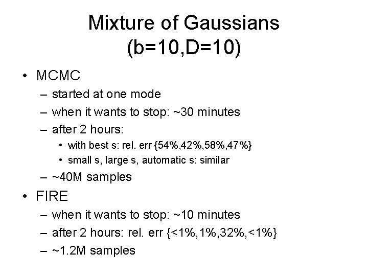
Mixture of Gaussians (b=10, D=10) • MCMC – started at one mode – when it wants to stop: ~30 minutes – after 2 hours: • with best s: rel. err {54%, 42%, 58%, 47%} • small s, large s, automatic s: similar – ~40 M samples • FIRE – when it wants to stop: ~10 minutes – after 2 hours: rel. err {<1%, 32%, <1%} – ~1. 2 M samples

Extension #1 Non-positive functions Positivization [Owen-Zhou 1998]

Extension #2 More defensiveness, and accuracy Control variates [Veach 1997]

Extension #3 More accurate regression Local linear regression

Extension #4 (maybe) Fully automatic stopping Function-wide confidence bands stitch together pointwise bands, control with FDR

Summary • We can do high-dimensional integration without Markov chains, by statistical inference • Promising alternative to MCMC – safer (e. g. isolated modes) – not a black art – faster • Intrinsic dimension - multiple viewpoints • MUCH more work needed – please help me!

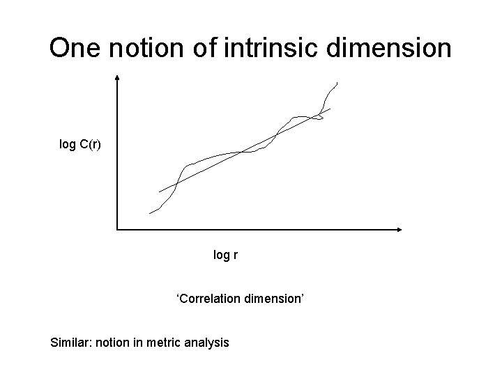
One notion of intrinsic dimension log C(r) log r ‘Correlation dimension’ Similar: notion in metric analysis

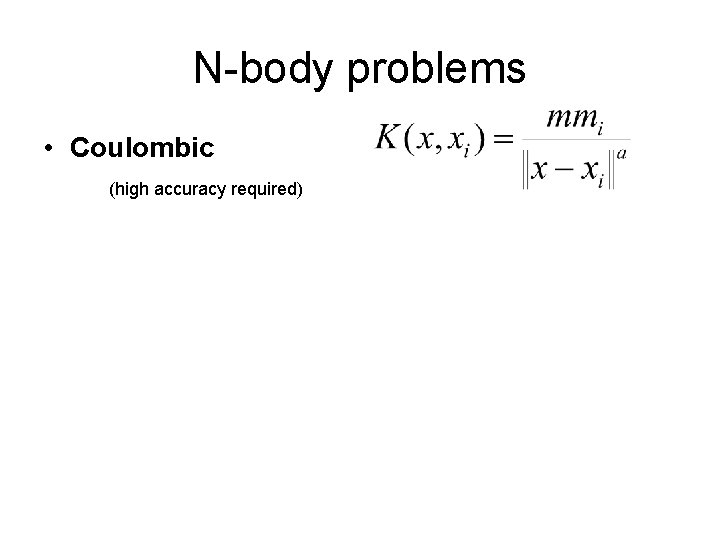
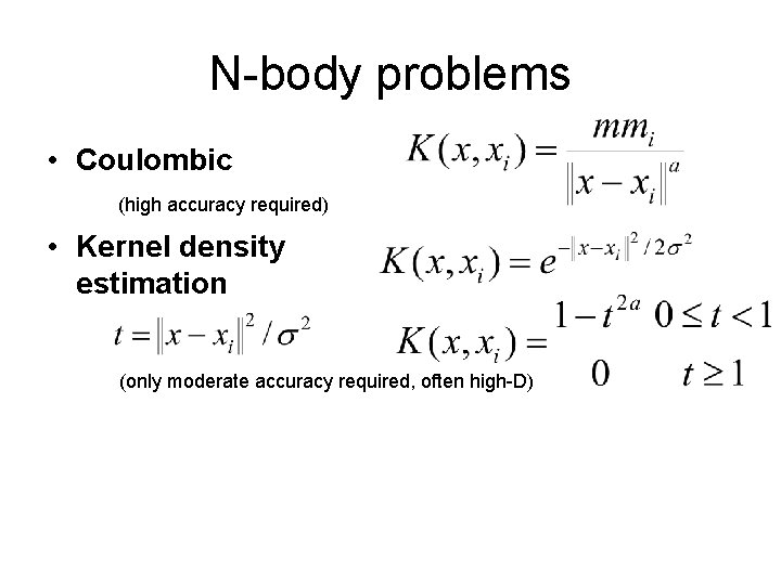
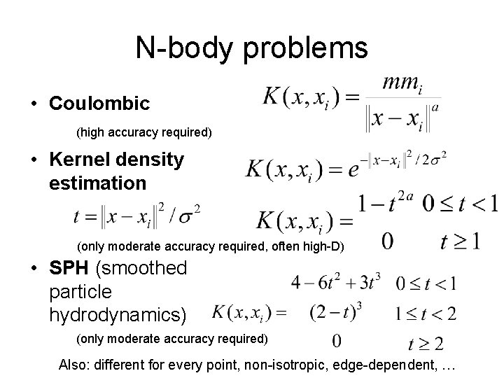
N-body problems • Coulombic (high accuracy required)

N-body problems • Coulombic (high accuracy required) • Kernel density estimation (only moderate accuracy required, often high-D)

N-body problems • Coulombic (high accuracy required) • Kernel density estimation (only moderate accuracy required, often high-D) • SPH (smoothed particle hydrodynamics) (only moderate accuracy required) Also: different for every point, non-isotropic, edge-dependent, …

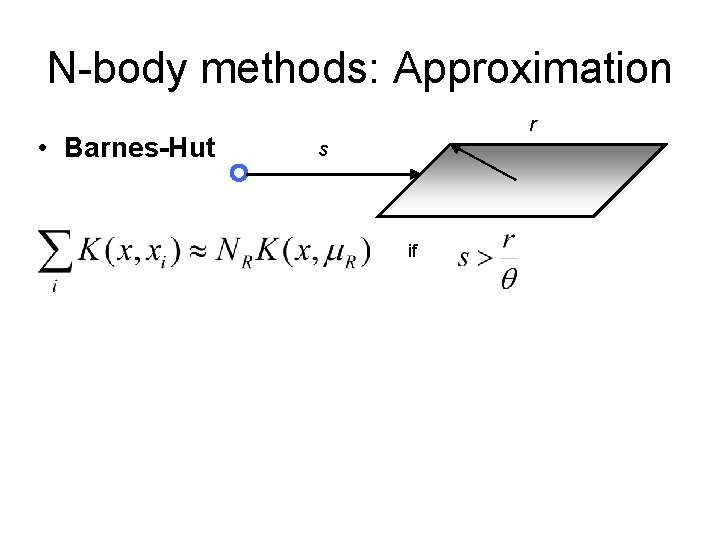
N-body methods: Approximation • Barnes-Hut r s if

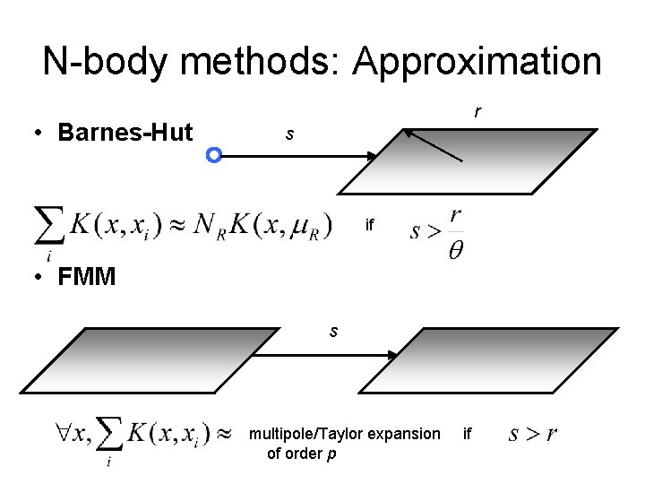
N-body methods: Approximation • Barnes-Hut r s if • FMM s multipole/Taylor expansion of order p if

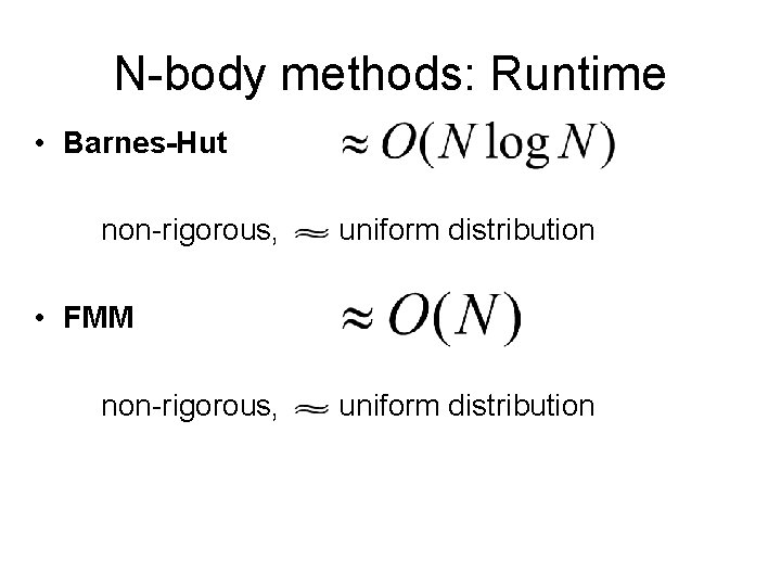
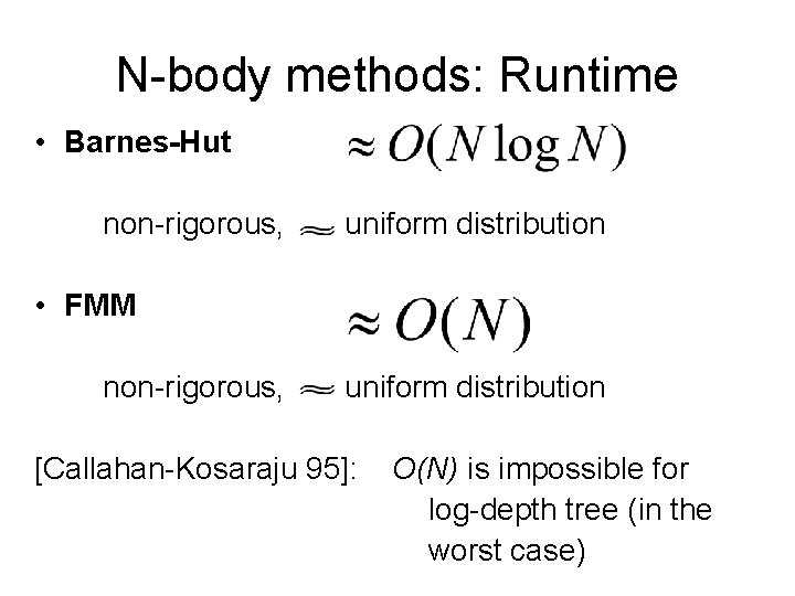
N-body methods: Runtime • Barnes-Hut non-rigorous, uniform distribution • FMM non-rigorous, uniform distribution

N-body methods: Runtime • Barnes-Hut non-rigorous, uniform distribution • FMM non-rigorous, uniform distribution [Callahan-Kosaraju 95]: O(N) is impossible for log-depth tree (in the worst case)

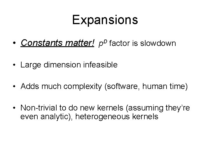
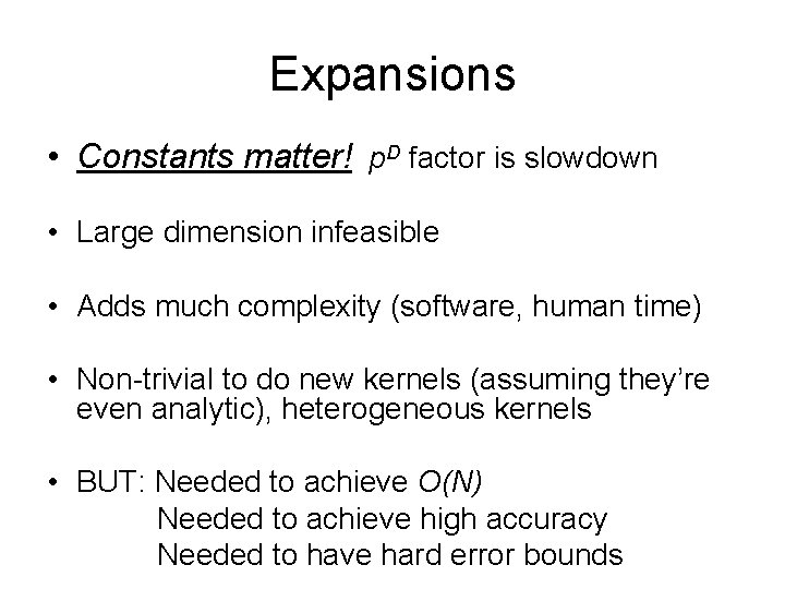
Expansions • Constants matter! p. D factor is slowdown • Large dimension infeasible • Adds much complexity (software, human time) • Non-trivial to do new kernels (assuming they’re even analytic), heterogeneous kernels

Expansions • Constants matter! p. D factor is slowdown • Large dimension infeasible • Adds much complexity (software, human time) • Non-trivial to do new kernels (assuming they’re even analytic), heterogeneous kernels • BUT: Needed to achieve O(N) Needed to achieve high accuracy Needed to have hard error bounds

Expansions • Constants matter! p. D factor is slowdown • Large dimension infeasible • Adds much complexity (software, human time) • Non-trivial to do new kernels (assuming they’re even analytic), heterogeneous kernels • BUT: Needed to achieve O(N) (? ) Needed to achieve high accuracy (? ) Needed to have hard error bounds (? )

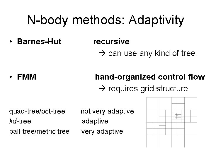
N-body methods: Adaptivity • Barnes-Hut recursive can use any kind of tree • FMM hand-organized control flow requires grid structure quad-tree/oct-tree kd-tree ball-tree/metric tree not very adaptive

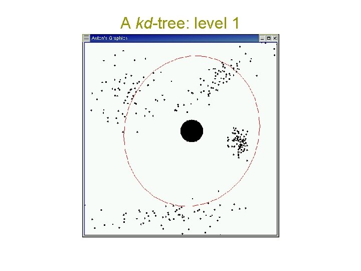
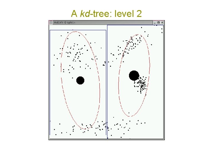
kd-trees: most widely-used spacepartitioning tree [Friedman, Bentley & Finkel 1977] • Univariate axis-aligned splits • Split on widest dimension • O(N log N) to build, O(N) space

A kd-tree: level 1

A kd-tree: level 2

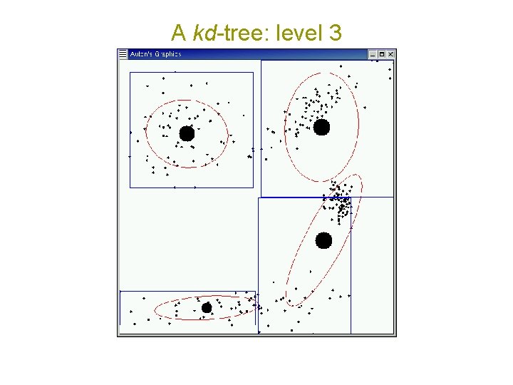
A kd-tree: level 3

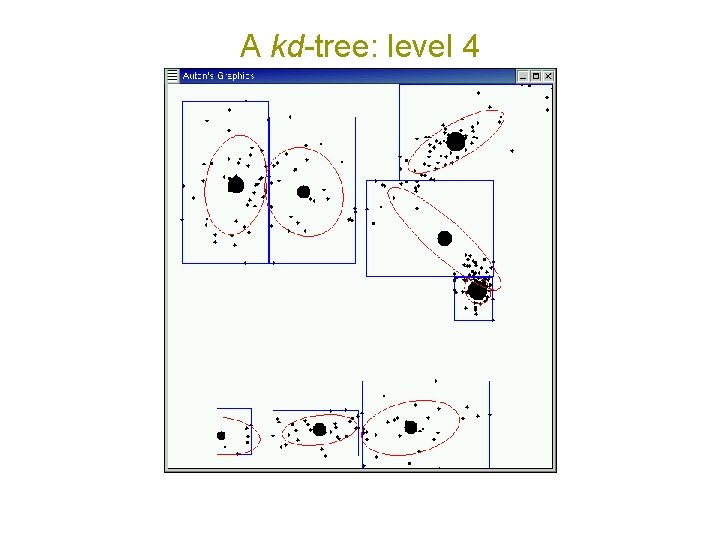
A kd-tree: level 4

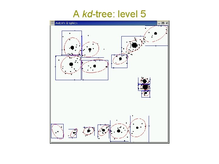
A kd-tree: level 5

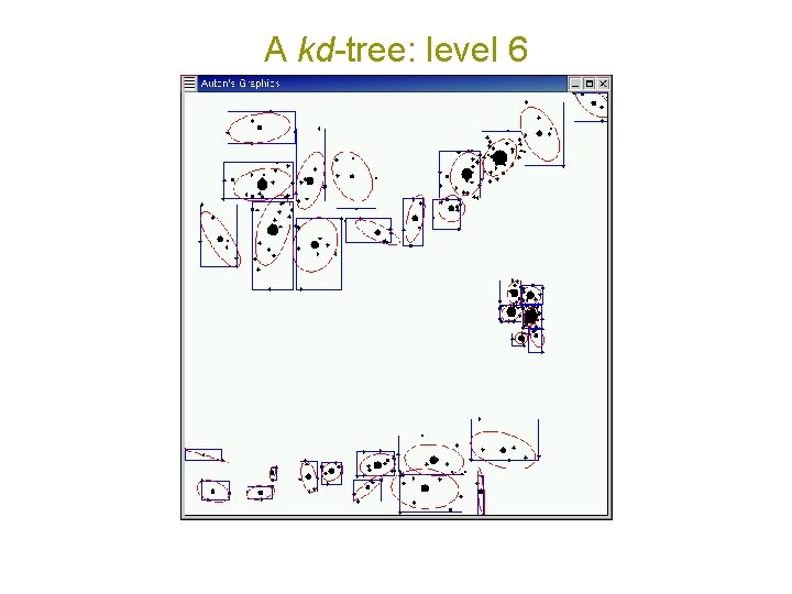
A kd-tree: level 6

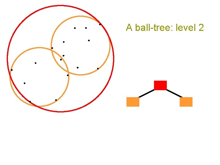
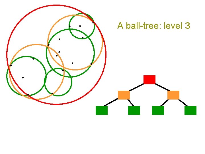
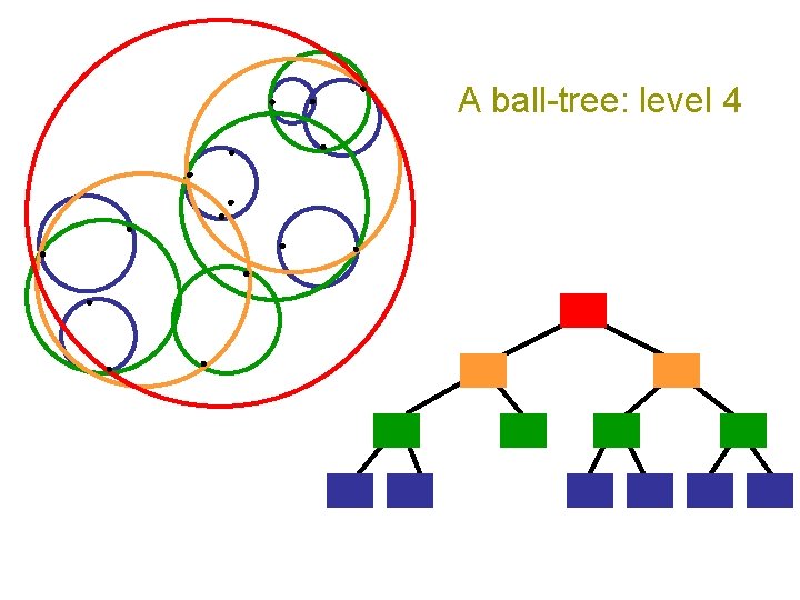
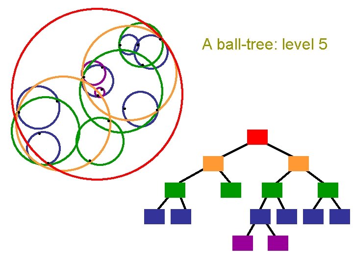
A ball-tree: level 1 [Uhlmann 1991], [Omohundro 1991]

A ball-tree: level 2

A ball-tree: level 3

A ball-tree: level 4

A ball-tree: level 5

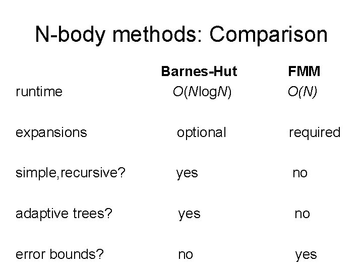
N-body methods: Comparison runtime Barnes-Hut O(Nlog. N) FMM O(N) expansions optional required simple, recursive? yes no adaptive trees? yes no error bounds? no yes

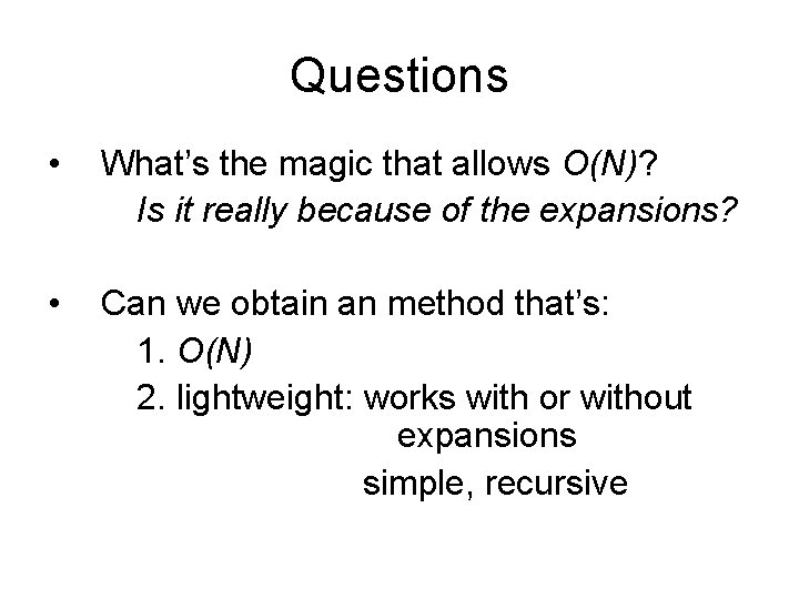
Questions • What’s the magic that allows O(N)? Is it really because of the expansions? • Can we obtain an method that’s: 1. O(N) 2. lightweight: works with or without. . . . expansions simple, recursive

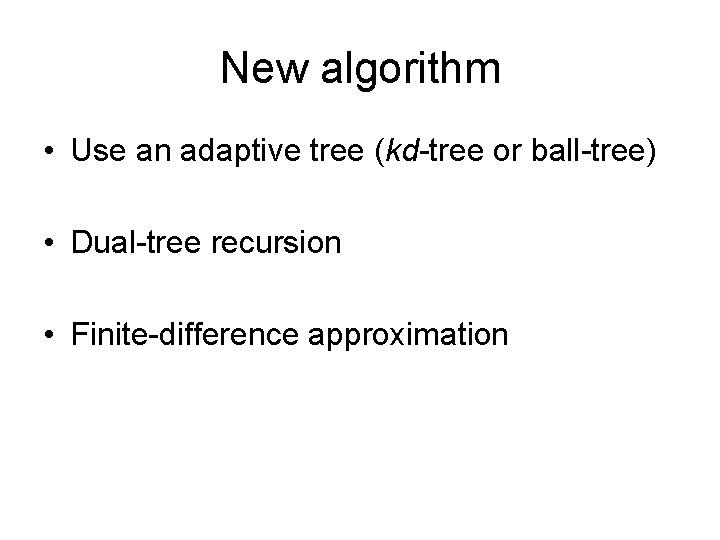
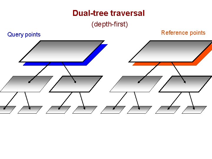
New algorithm • Use an adaptive tree (kd-tree or ball-tree) • Dual-tree recursion • Finite-difference approximation

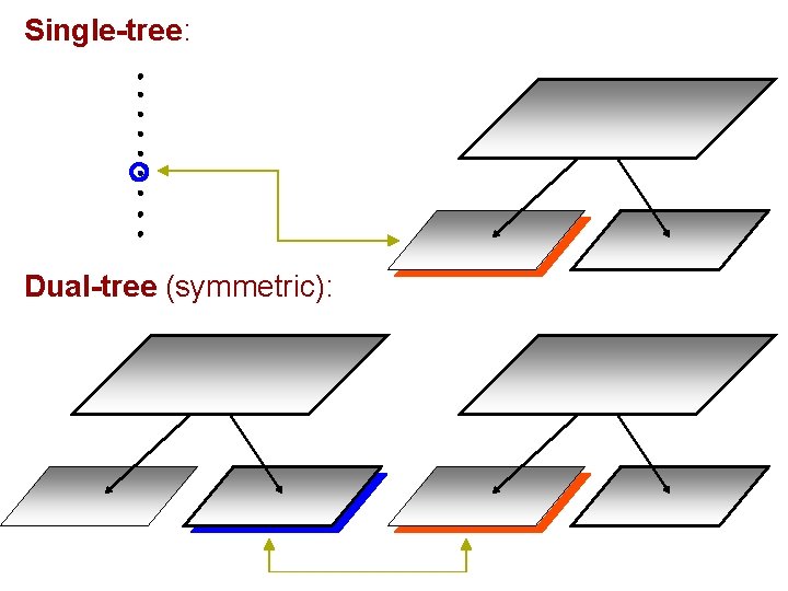
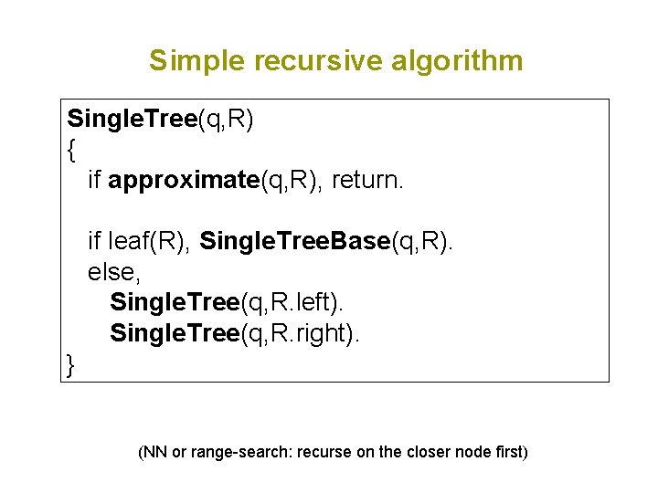
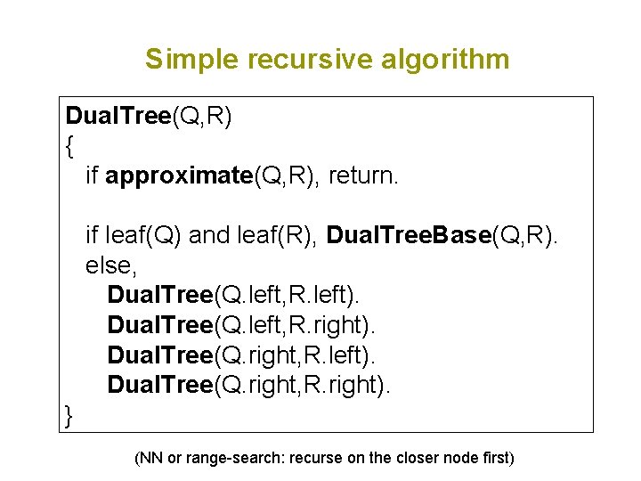
Single-tree: Dual-tree (symmetric):

Simple recursive algorithm Single. Tree(q, R) { if approximate(q, R), return. if leaf(R), Single. Tree. Base(q, R). else, Single. Tree(q, R. left). Single. Tree(q, R. right). } (NN or range-search: recurse on the closer node first)

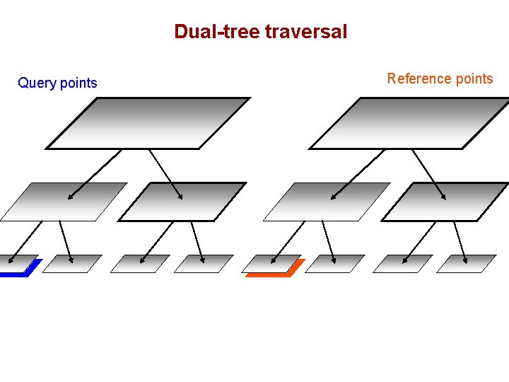
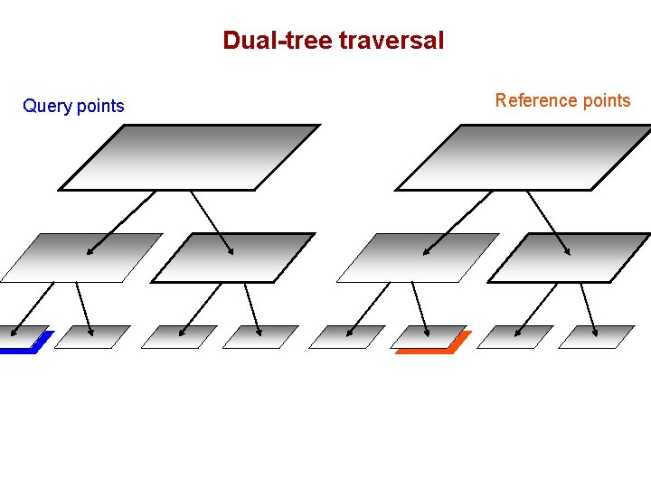
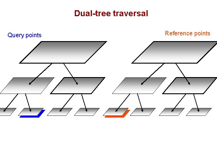
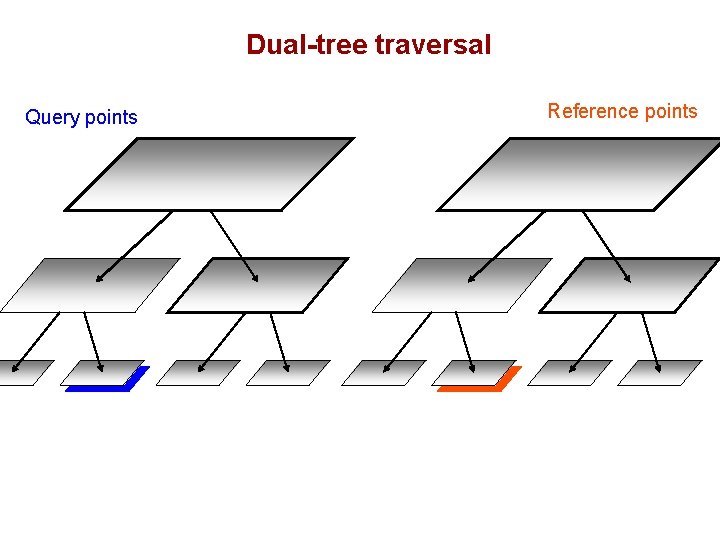
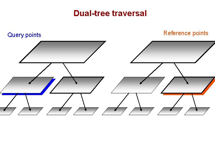
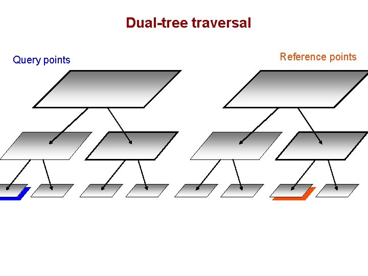
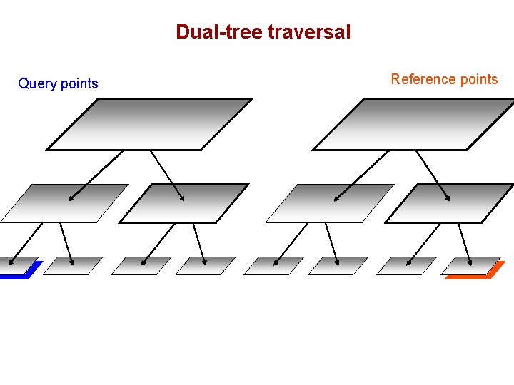
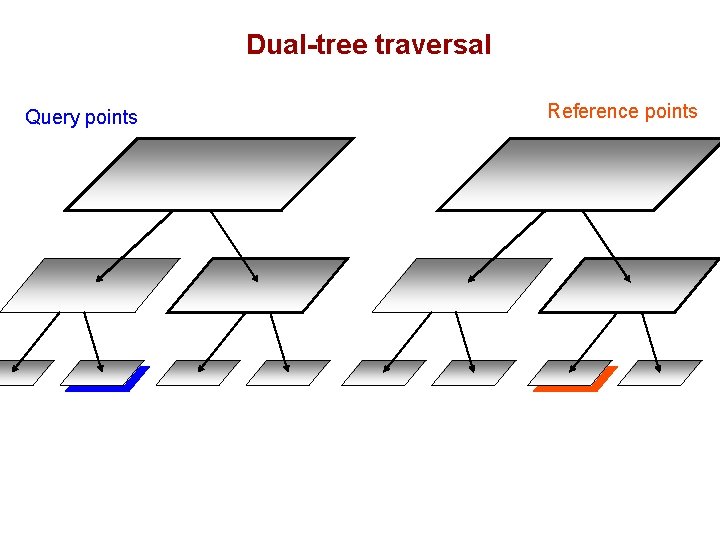
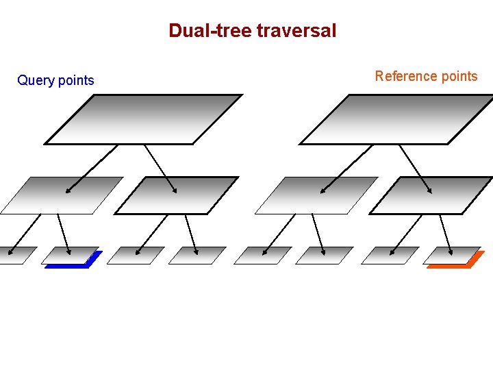
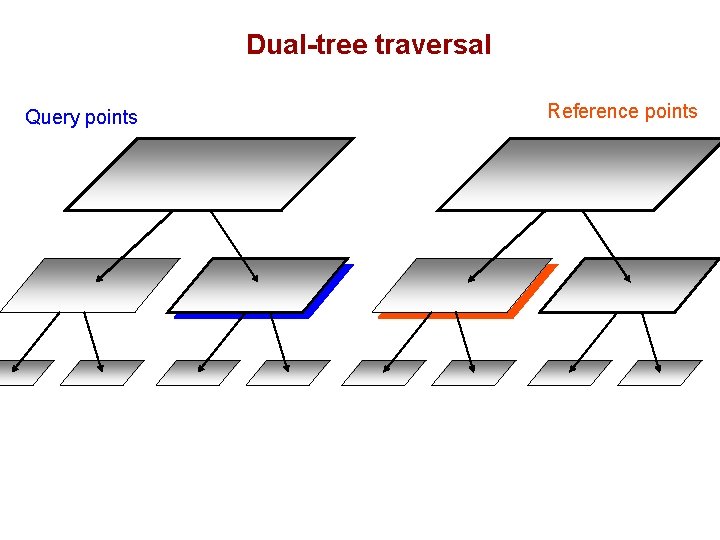
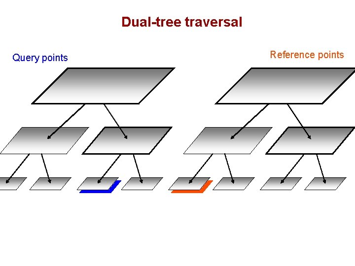
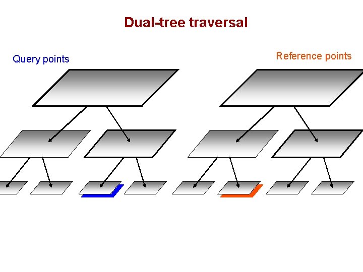
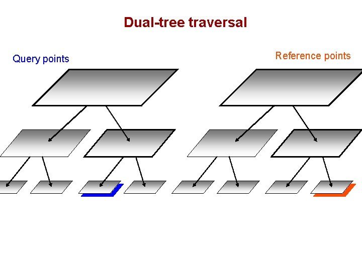
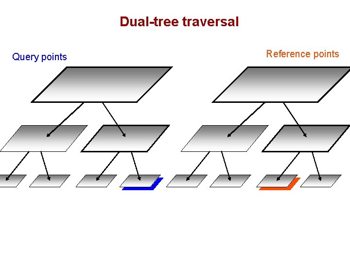
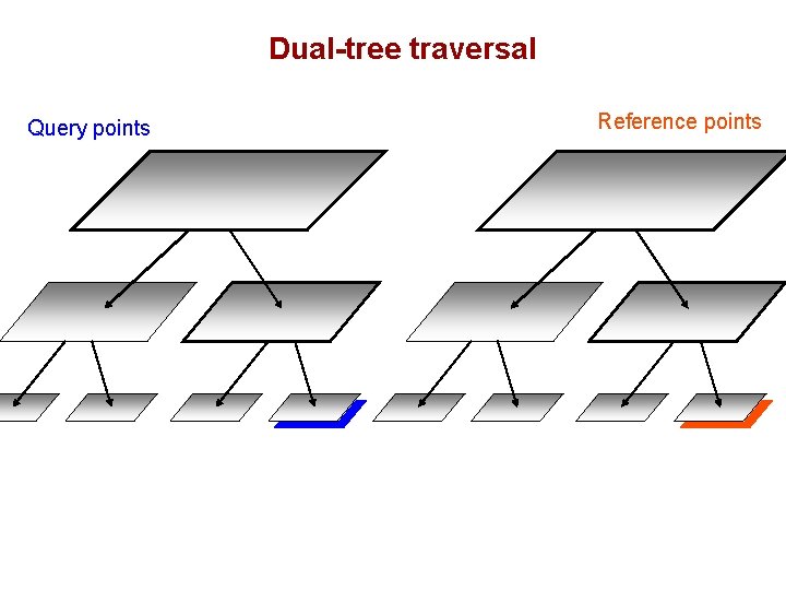
Simple recursive algorithm Dual. Tree(Q, R) { if approximate(Q, R), return. if leaf(Q) and leaf(R), Dual. Tree. Base(Q, R). else, Dual. Tree(Q. left, R. left). Dual. Tree(Q. left, R. right). Dual. Tree(Q. right, R. left). Dual. Tree(Q. right, R. right). } (NN or range-search: recurse on the closer node first)

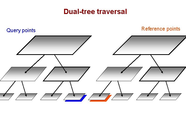
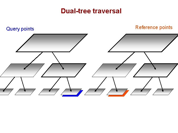
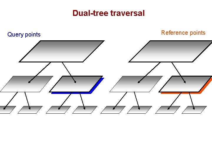
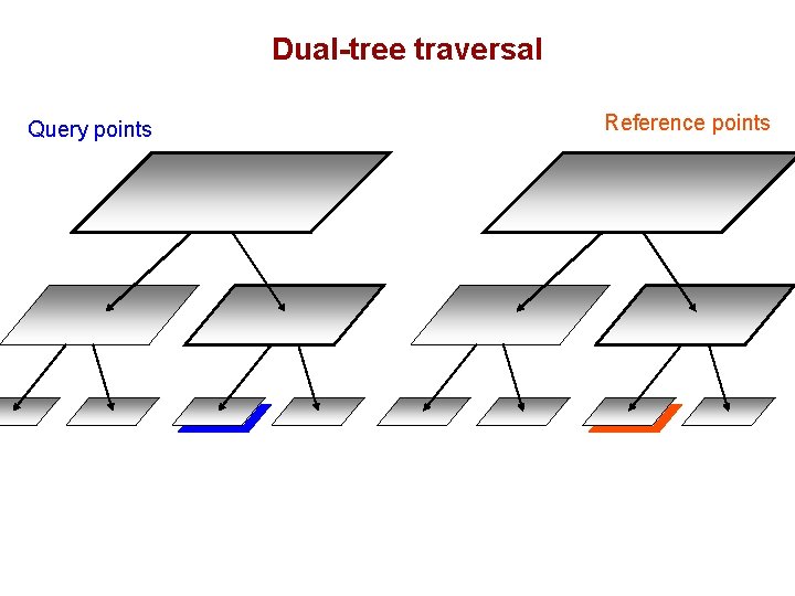
Dual-tree traversal (depth-first) Query points Reference points

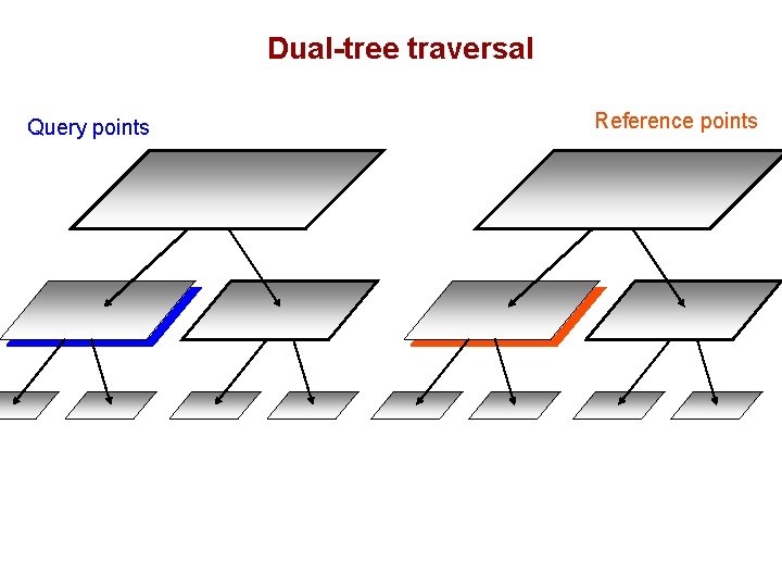
Dual-tree traversal Query points Reference points

Dual-tree traversal Query points Reference points

Dual-tree traversal Query points Reference points

Dual-tree traversal Query points Reference points

Dual-tree traversal Query points Reference points

Dual-tree traversal Query points Reference points

Dual-tree traversal Query points Reference points

Dual-tree traversal Query points Reference points

Dual-tree traversal Query points Reference points

Dual-tree traversal Query points Reference points

Dual-tree traversal Query points Reference points

Dual-tree traversal Query points Reference points

Dual-tree traversal Query points Reference points

Dual-tree traversal Query points Reference points

Dual-tree traversal Query points Reference points

Dual-tree traversal Query points Reference points

Dual-tree traversal Query points Reference points

Dual-tree traversal Query points Reference points

Dual-tree traversal Query points Reference points

Dual-tree traversal Query points Reference points

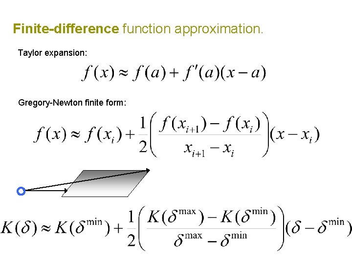
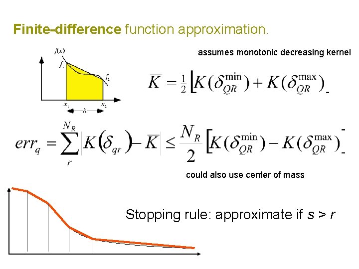
Finite-difference function approximation. Taylor expansion: Gregory-Newton finite form:

Finite-difference function approximation. assumes monotonic decreasing kernel could also use center of mass Stopping rule: approximate if s > r

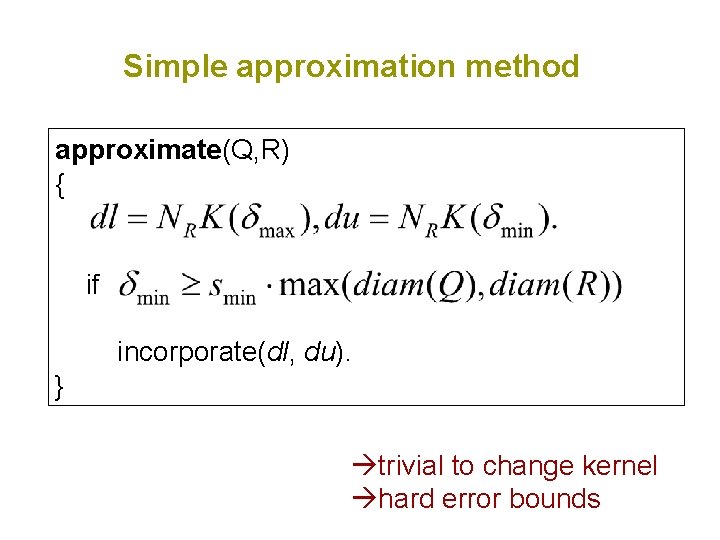
Simple approximation method approximate(Q, R) { if incorporate(dl, du). } trivial to change kernel hard error bounds

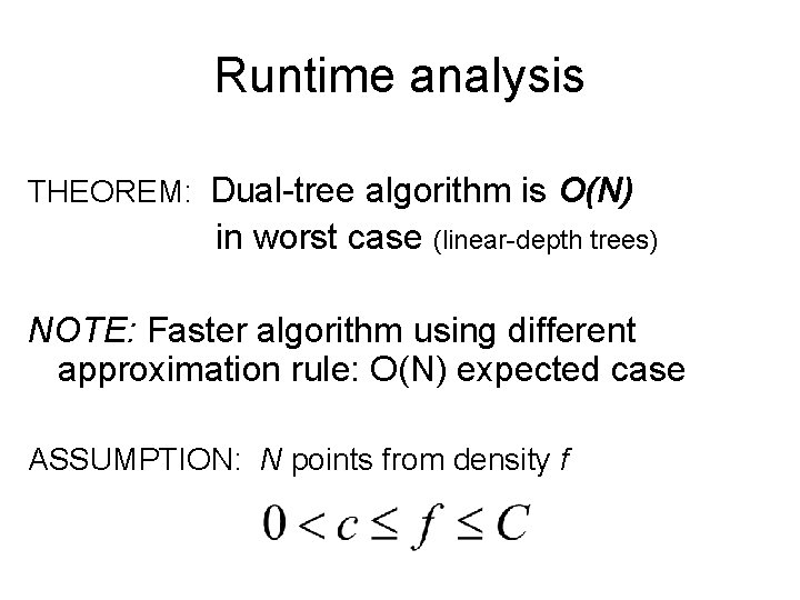
Runtime analysis THEOREM: Dual-tree algorithm is O(N) in worst case (linear-depth trees) NOTE: Faster algorithm using different approximation rule: O(N) expected case ASSUMPTION: N points from density f

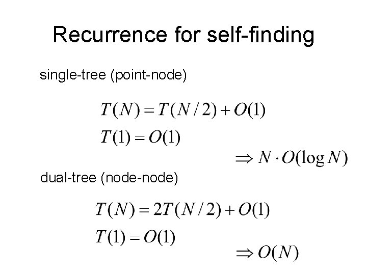
Recurrence for self-finding single-tree (point-node) dual-tree (node-node)

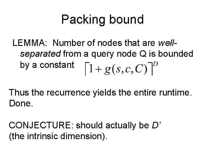
Packing bound LEMMA: Number of nodes that are wellseparated from a query node Q is bounded by a constant Thus the recurrence yields the entire runtime. Done. CONJECTURE: should actually be D’ (the intrinsic dimension).

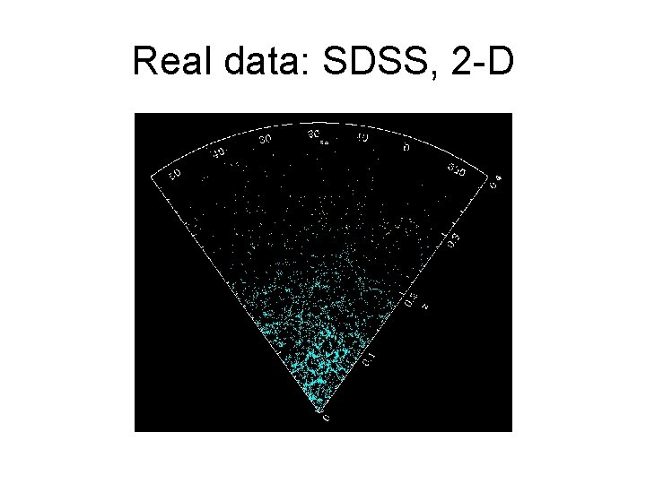
Real data: SDSS, 2 -D

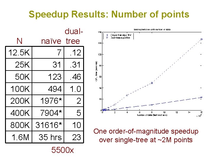
Speedup Results: Number of points N naïve 12. 5 K 7 25 K 31 50 K 123 100 K 494 200 K 1976* 400 K 7904* 800 K 31616* 1. 6 M 35 hrs dualtree. 12. 31. 46 1. 0 2 5 10 23 5500 x One order-of-magnitude speedup over single-tree at ~2 M points

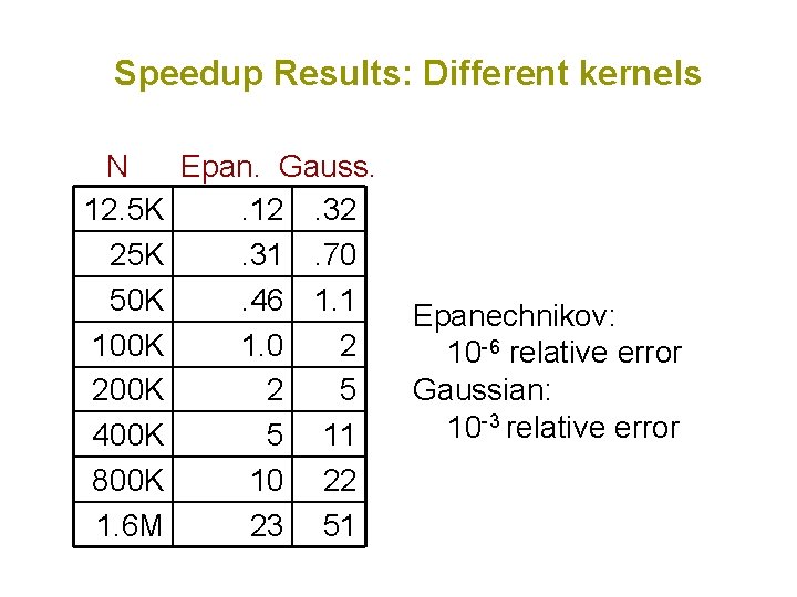
Speedup Results: Different kernels N Epan. Gauss. 12. 5 K. 12. 32 25 K. 31. 70 50 K. 46 1. 1 100 K 1. 0 2 200 K 2 5 400 K 5 11 800 K 10 22 1. 6 M 23 51 Epanechnikov: 10 -6 relative error Gaussian: 10 -3 relative error

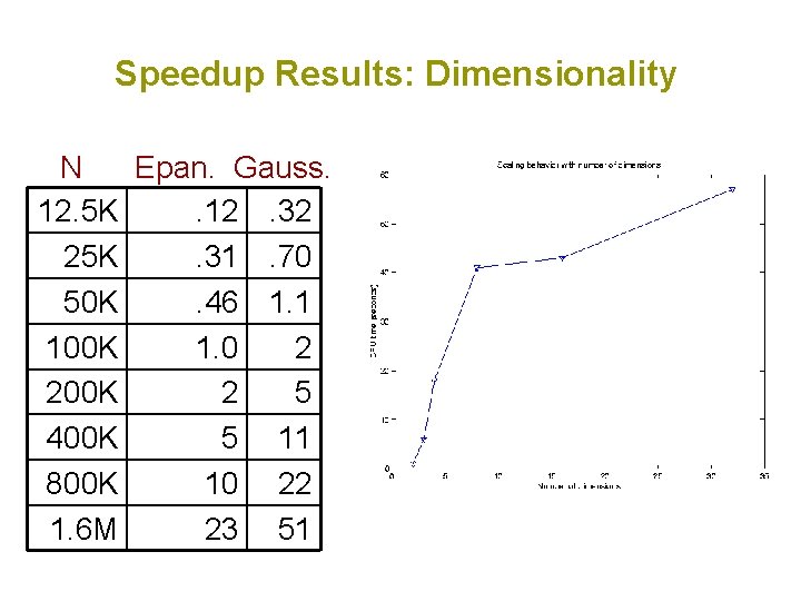
Speedup Results: Dimensionality N Epan. Gauss. 12. 5 K. 12. 32 25 K. 31. 70 50 K. 46 1. 1 100 K 1. 0 2 200 K 2 5 400 K 5 11 800 K 10 22 1. 6 M 23 51

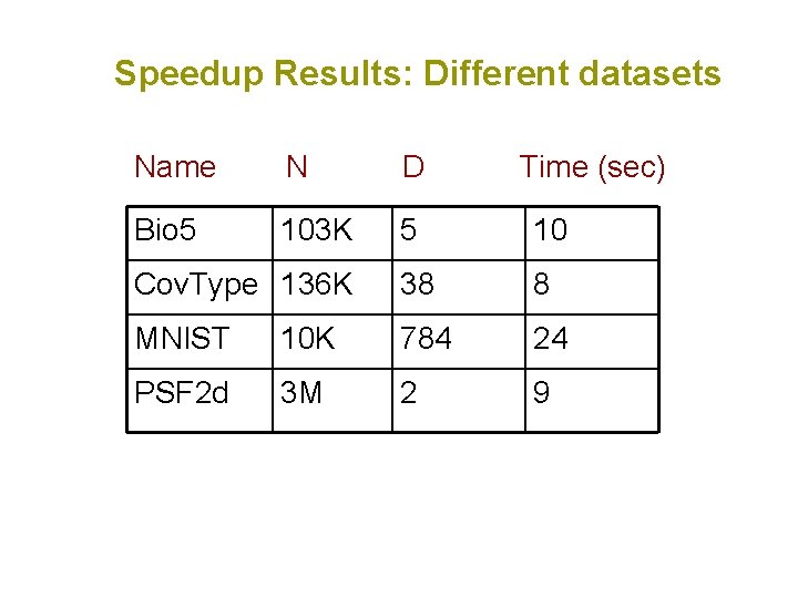
Speedup Results: Different datasets Name N D Time (sec) Bio 5 103 K 5 10 Cov. Type 136 K 38 8 MNIST 10 K 784 24 PSF 2 d 3 M 2 9

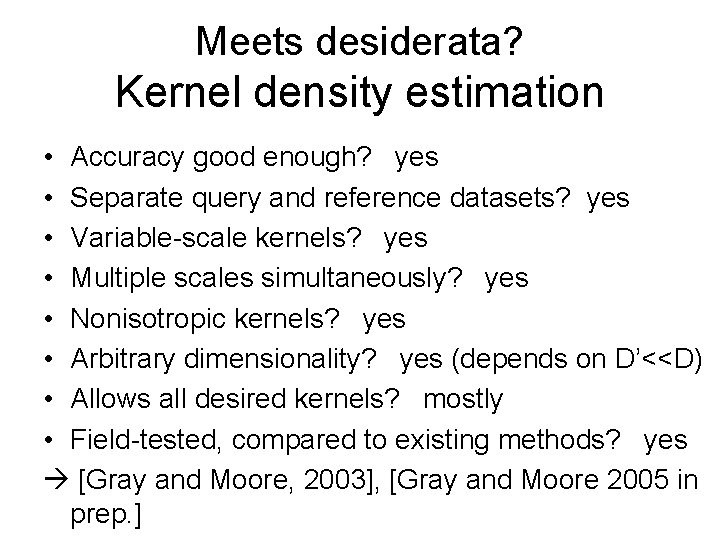
Meets desiderata? Kernel density estimation • Accuracy good enough? yes • Separate query and reference datasets? yes • Variable-scale kernels? yes • Multiple scales simultaneously? yes • Nonisotropic kernels? yes • Arbitrary dimensionality? yes (depends on D’<<D) • Allows all desired kernels? mostly • Field-tested, compared to existing methods? yes [Gray and Moore, 2003], [Gray and Moore 2005 in prep. ]

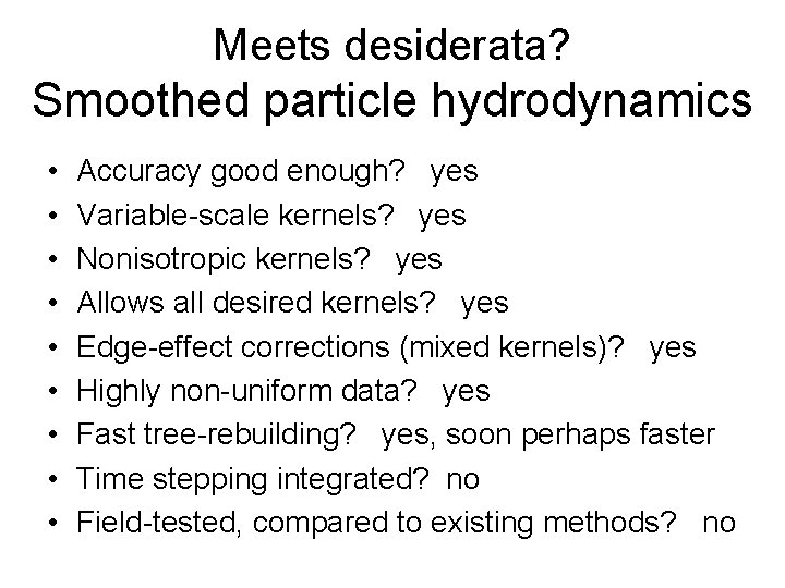
Meets desiderata? Smoothed particle hydrodynamics • • • Accuracy good enough? yes Variable-scale kernels? yes Nonisotropic kernels? yes Allows all desired kernels? yes Edge-effect corrections (mixed kernels)? yes Highly non-uniform data? yes Fast tree-rebuilding? yes, soon perhaps faster Time stepping integrated? no Field-tested, compared to existing methods? no

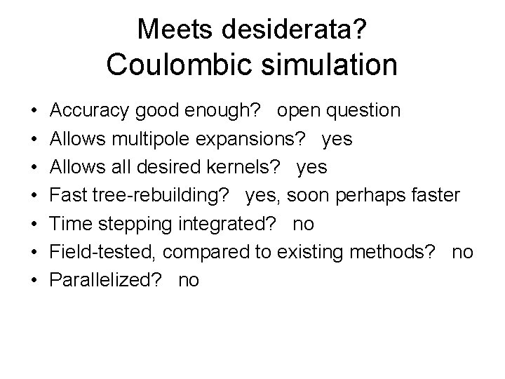
Meets desiderata? Coulombic simulation • • Accuracy good enough? open question Allows multipole expansions? yes Allows all desired kernels? yes Fast tree-rebuilding? yes, soon perhaps faster Time stepping integrated? no Field-tested, compared to existing methods? no Parallelized? no

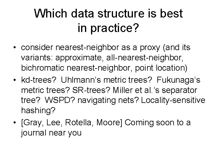
Which data structure is best in practice? • consider nearest-neighbor as a proxy (and its variants: approximate, all-nearest-neighbor, bichromatic nearest-neighbor, point location) • kd-trees? Uhlmann’s metric trees? Fukunaga’s metric trees? SR-trees? Miller et al. ’s separator tree? WSPD? navigating nets? Locality-sensitive hashing? • [Gray, Lee, Rotella, Moore] Coming soon to a journal near you

Side note: Many problems are easy for this framework • • Correlation dimension Hausdorff distance Euclidean minimum spanning tree more

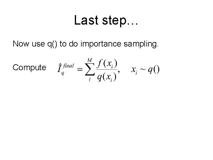
Last step… Now use q() to do importance sampling. Compute