
High Throughput Sequencing Technologies Applications Michael Brudno CSC
High Throughput Sequencing: Technologies & Applications Michael Brudno CSC 2431 – Algorithms for HTS University of Toronto 06/01/2010
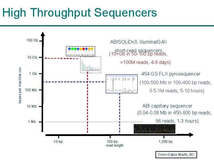
High Throughput Sequencers 100 Gb AB/SOLi. Dv 3, Illumina/GAII short-read sequencers (10+Gb in 50 -100 bp reads, 10 Gb bases per machine run >100 M reads, 4 -8 days) 454 GS FLX pyrosequencer 1 Gb (100 -500 Mb in 100 -400 bp reads, 100 Mb 0. 5 -1 M reads, 5 -10 hours) ABI capillary sequencer (0. 04 -0. 08 Mb in 450 -800 bp reads, 10 Mb 96 reads, 1 -3 hours) 1 Mb 10 bp 100 bp read length 1, 000 bp From Gabor Marth, BC
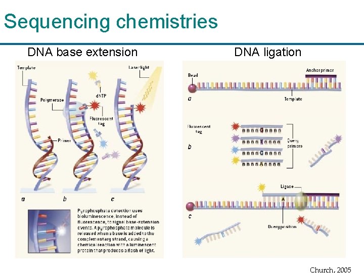
Sequencing chemistries DNA base extension DNA ligation Church, 2005
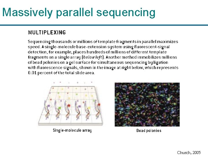
Massively parallel sequencing Church, 2005
Features of HTS data • Short (for now) sequence reads – 200 -400 bp: 454 (Roche) – 35 -100 bp Solexa(Illumina), SOLi. D(AB) • Huge amount of sequence per run –Up to 10 s of gigabases per run • Huge number of reads per run –Up to 100’s of millions • Higher error (compared with Sanger) –Different error profile
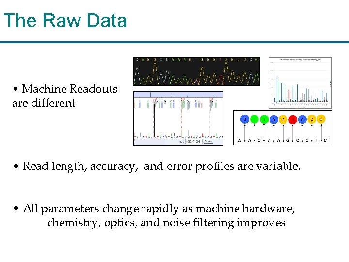
The Raw Data • Machine Readouts are different • Read length, accuracy, and error profiles are variable. • All parameters change rapidly as machine hardware, chemistry, optics, and noise filtering improves
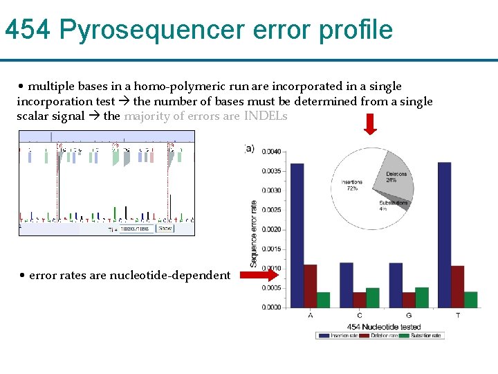
454 Pyrosequencer error profile • multiple bases in a homo-polymeric run are incorporated in a single incorporation test the number of bases must be determined from a single scalar signal the majority of errors are INDELs • error rates are nucleotide-dependent
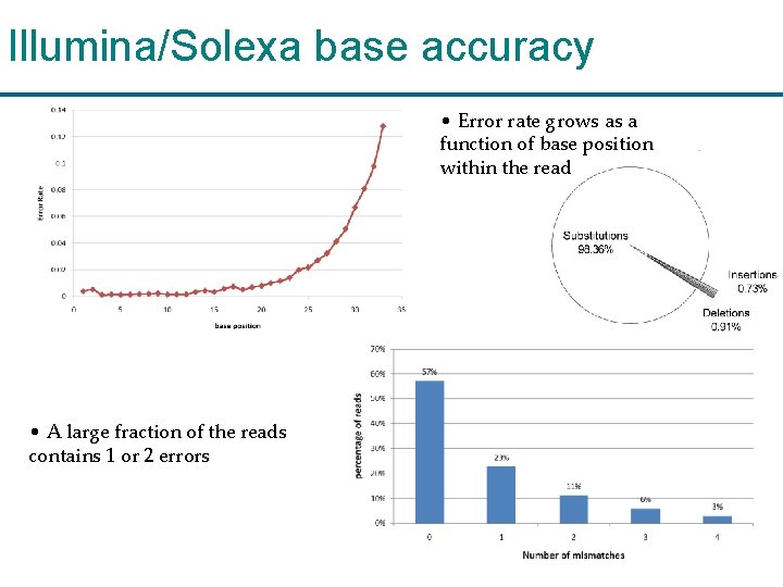
Illumina/Solexa base accuracy • Error rate grows as a function of base position within the read • A large fraction of the reads contains 1 or 2 errors
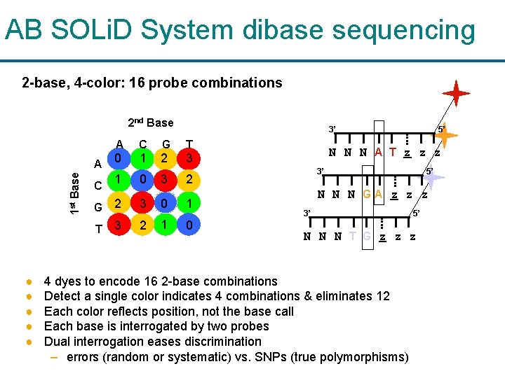
AB SOLi. D System dibase sequencing 2 -base, 4 -color: 16 probe combinations 1 st Base 2 nd Base ● ● ● 3’ A C G T A 0 1 C 1 2 3 0 3 2 G 2 3 0 1 T 3 2 1 0 5’ N N N A T z z z 3’ 5’ N N N GA z z z 3’ 5’ N N N T G z z z 4 dyes to encode 16 2 -base combinations Detect a single color indicates 4 combinations & eliminates 12 Each color reflects position, not the base call Each base is interrogated by two probes Dual interrogation eases discrimination – errors (random or systematic) vs. SNPs (true polymorphisms)
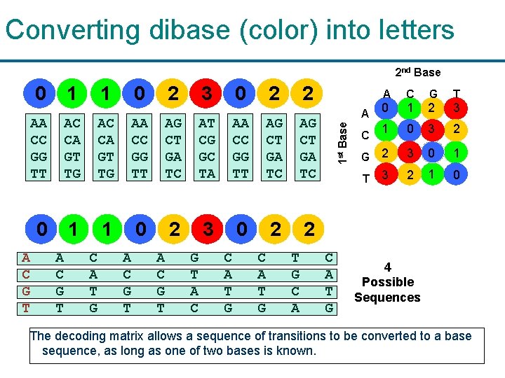
Converting dibase (color) into letters 2 nd Base 1 0 1 2 3 0 2 2 AA CC GG TT AC CA GT TG AA CC GG TT AG CT GA TC AT CG GC TA AA CC GG TT AG CT GA TC 0 1 1 0 2 3 0 2 2 A C G T C A T G A C G T G T A C C A T G T G C A A C G T 0 1 2 3 1 0 3 2 G 2 3 0 1 T 3 2 1 0 A 1 st Base 0 C A T G C 4 Possible Sequences The decoding matrix allows a sequence of transitions to be converted to a base sequence, as long as one of two bases is known.
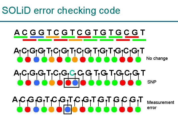
SOLi. D error checking code ACGGTCGTCGTGTGCGT No change ACGGTCGCCGTGTGCGT SNP ACGGTCGTCGTGTGCGT Measurement error

SOLi. D Error rate & QVs
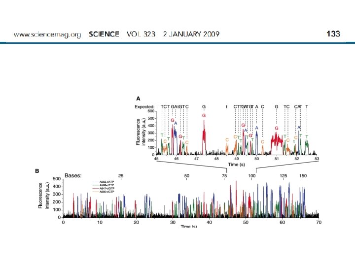
Pacific Biosystems (Pac. Bio)
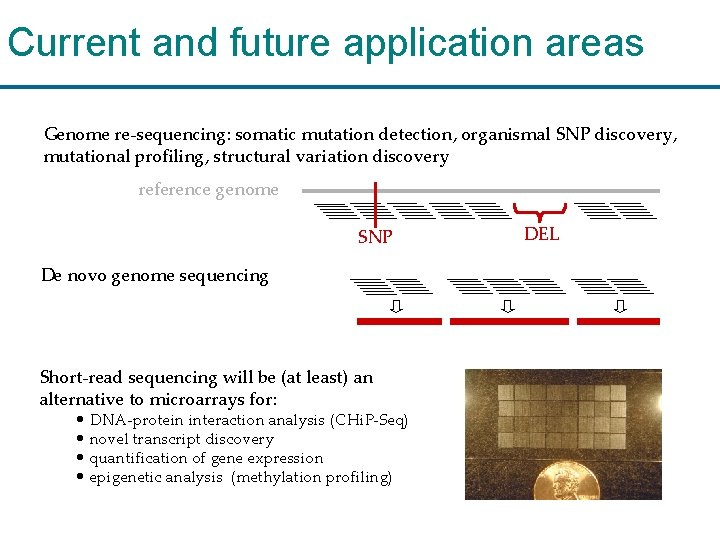
Current and future application areas Genome re-sequencing: somatic mutation detection, organismal SNP discovery, mutational profiling, structural variation discovery reference genome SNP De novo genome sequencing Short-read sequencing will be (at least) an alternative to microarrays for: • DNA-protein interaction analysis (CHi. P-Seq) • novel transcript discovery • quantification of gene expression • epigenetic analysis (methylation profiling) DEL
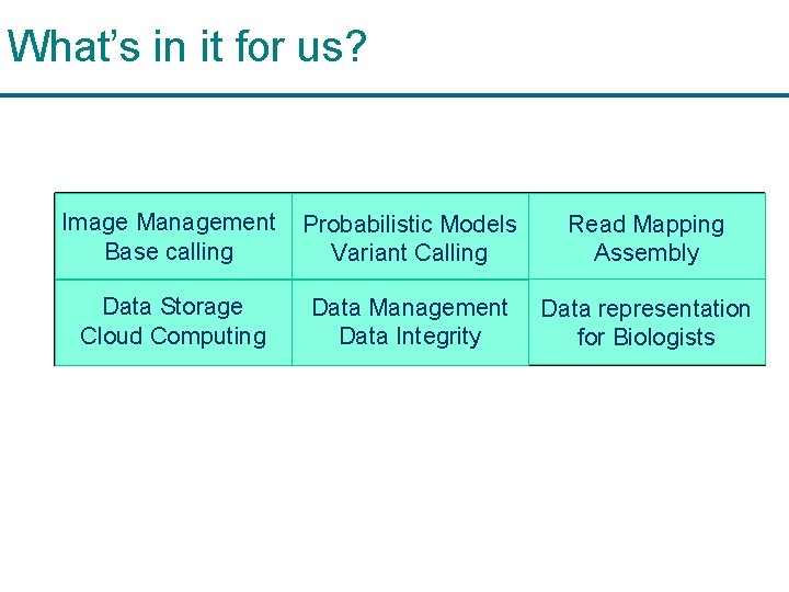
What’s in it for us? Image Management VISION/Graphics Base calling Probabilistic Models Machine Learning Variant Calling Read Mapping String Algorithms Assembly Data Storage Systems Cloud Computing Data Management Databases Data Integrity Data representation Human-Computer for. Interaction Biologists
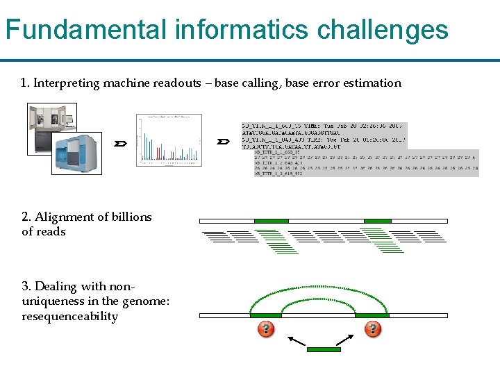
Fundamental informatics challenges 1. Interpreting machine readouts – base calling, base error estimation 2. Alignment of billions of reads 3. Dealing with nonuniqueness in the genome: resequenceability
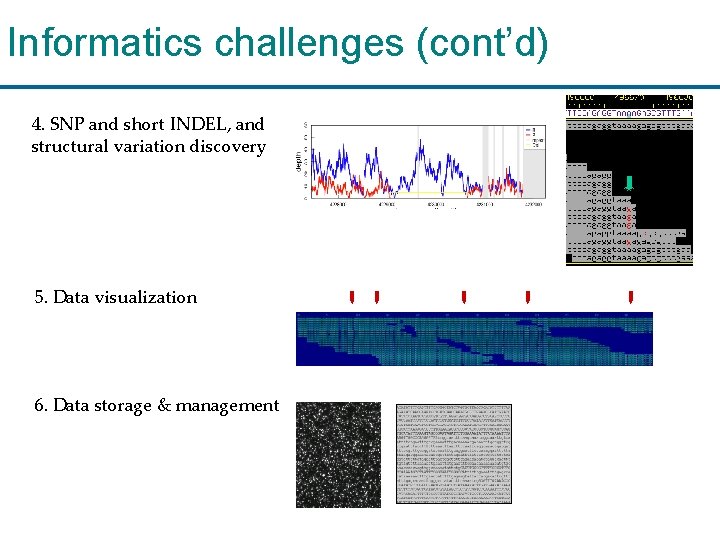
Informatics challenges (cont’d) 4. SNP and short INDEL, and structural variation discovery 5. Data visualization 6. Data storage & management
High Throughput Sequencing: Technologies & Applications Questions?
SHRi. MP: SHort Read Mapping Package • Fast Mapping Algorithm - Spaced seed hashing - Vectored (very fast) Smith Waterman - Handles micro insertions/deletions • Specialized algorithm for aligning color-space (AB SOLi. D) reads • Computes p-values (and other statistics)
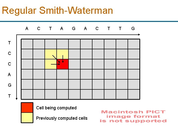
Regular Smith-Waterman A C T A G A T C C A G T Cell being computed Previously computed cells C T T G
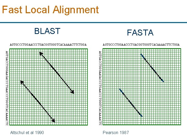
Fast Local Alignment BLAST FASTA AGTGCCCTGGAACCCTGACGGTGGGTCACAAAACTTCTGGA AGTGACCTGGGAAGACCCTGAACCCTGGGTCACAAAACTC Altschul et al 1990 Pearson 1987
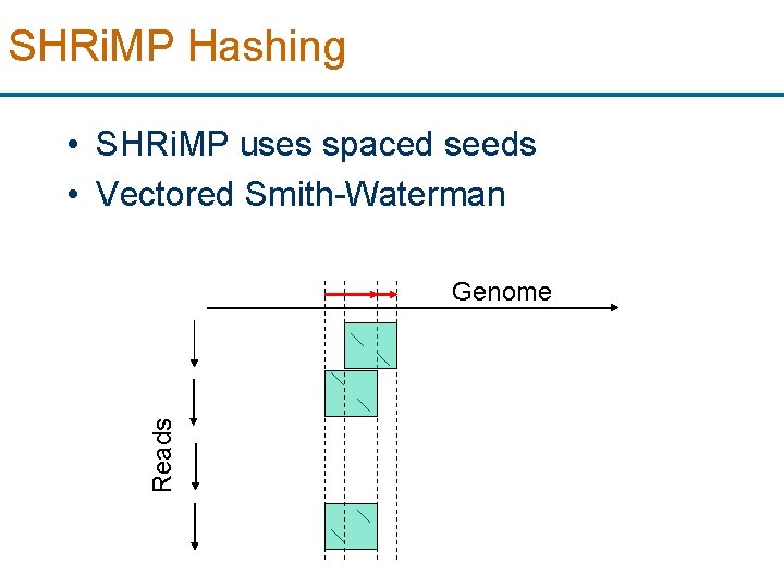
SHRi. MP Hashing • SHRi. MP uses spaced seeds • Vectored Smith-Waterman Reads Genome
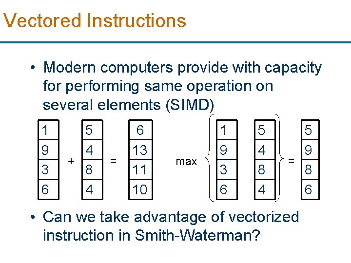
Vectored Instructions • Modern computers provide with capacity for performing same operation on several elements (SIMD) 1 9 3 6 5 4 + 8 4 = 6 13 11 10 max 1 9 3 6 5 4 8 4 5 9 = 8 6 • Can we take advantage of vectorized instruction in Smith-Waterman?
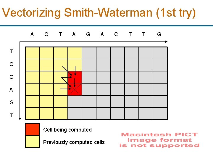
Vectorizing Smith-Waterman (1 st try) A C T A G A T C C A G T Cell being computed Previously computed cells C T T G
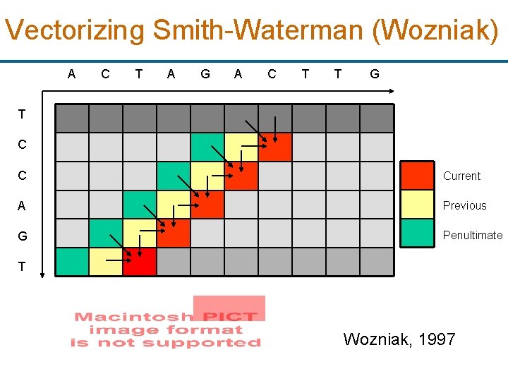
Vectorizing Smith-Waterman (Wozniak) A C T A G A C T T G T C C Current A Previous G Penultimate T Wozniak, 1997
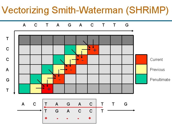
Vectorizing Smith-Waterman (SHRi. MP) A C T A G A C T T G T + C - C Current - A Previous - G Penultimate + T A C T A G A C T T G A C C T + - - - + T G
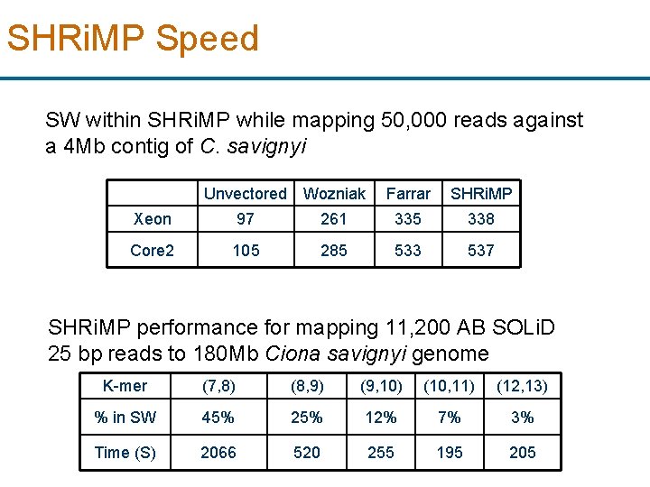
SHRi. MP Speed SW within SHRi. MP while mapping 50, 000 reads against a 4 Mb contig of C. savignyi Unvectored Wozniak Farrar SHRi. MP Xeon 97 261 335 338 Core 2 105 285 533 537 SHRi. MP performance for mapping 11, 200 AB SOLi. D 25 bp reads to 180 Mb Ciona savignyi genome K-mer (7, 8) (8, 9) (9, 10) (10, 11) (12, 13) % in SW 45% 25% 12% 7% 3% Time (S) 2066 520 255 195 205
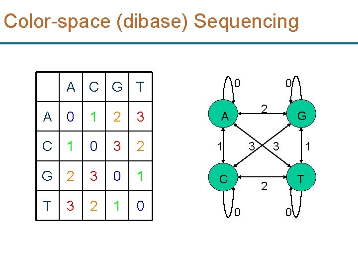
Color-space (dibase) Sequencing 0 A C G T A 0 1 2 3 C 1 0 3 2 1 G 2 3 0 1 C T 3 2 1 0 0 2 A 3 G 3 1 T 2 0 0
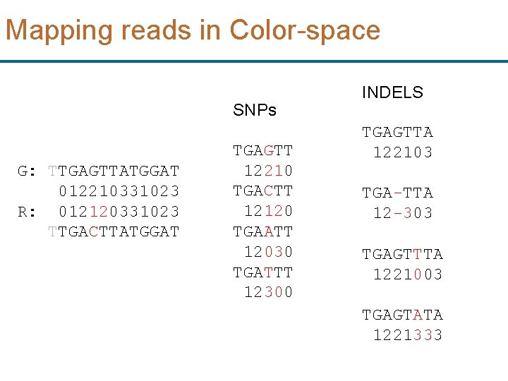
Mapping reads in Color-space SNPs G: TTGAGTTATGGAT 012210331023 R: 012120331023 TTGACTTATGGAT TGAGTT 12210 TGACTT 12120 TGAATT 12030 TGATTT 12300 INDELS TGAGTTA 122103 TGA-TTA 12 -303 TGAGTTTA 1221003 TGAGTATA 1221333
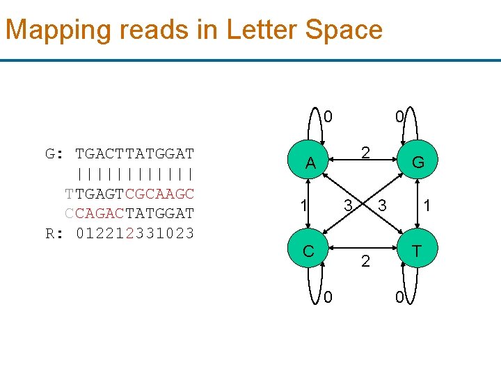
Mapping reads in Letter Space 0 G: TGACTTATGGAT |||||| TTGAGTCGCAAGC CCAGACTATGGAT R: 012212331023 0 2 A 1 3 C G 3 1 T 2 0 0
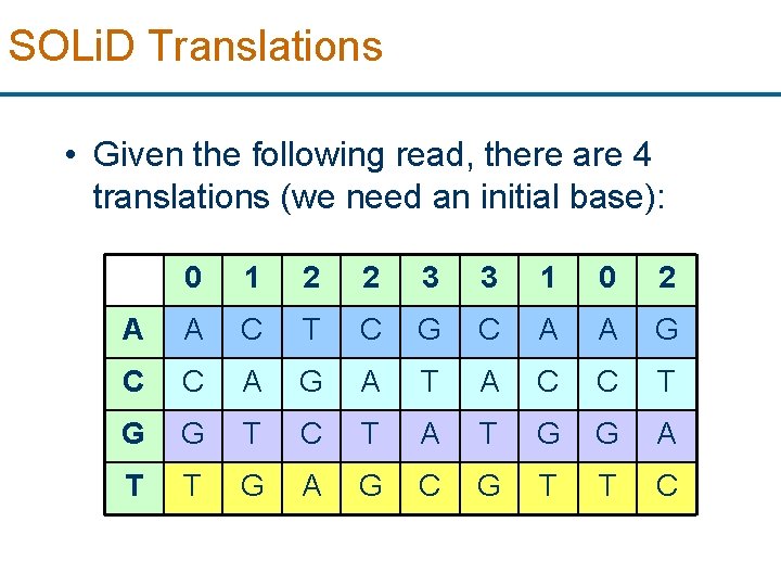
SOLi. D Translations • Given the following read, there are 4 translations (we need an initial base): 0 1 2 2 3 3 1 0 2 A A C T C G C A A G C C A G A T A C C T G G T C T A T G G A T T G A G C G T T C
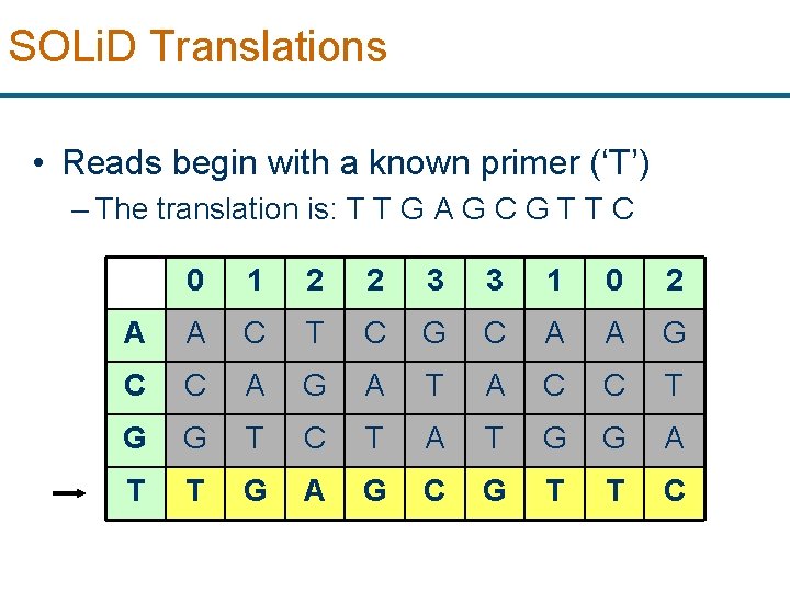
SOLi. D Translations • Reads begin with a known primer (‘T’) – The translation is: T T G A G C G T T C 0 1 2 2 3 3 1 0 2 A A C T C G C A A G C C A G A T A C C T G G T C T A T G G A T T G A G C G T T C
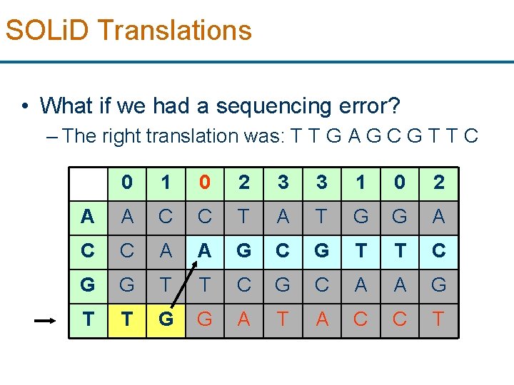
SOLi. D Translations • What if we had a sequencing error? – The right translation was: T T G A G C G T T C 0 1 0 2 3 3 1 0 2 A A C C T A T G G A C C A A G C G T T C G C A A G T T G G A T A C C T
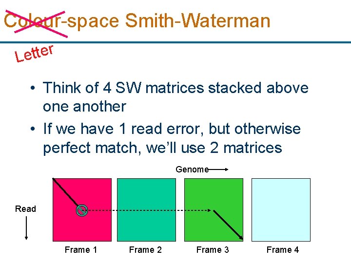
Colour-space Smith-Waterman r e t t e L • Think of 4 SW matrices stacked above one another • If we have 1 read error, but otherwise perfect match, we’ll use 2 matrices Genome Read Frame 1 Frame 2 Frame 3 Frame 4
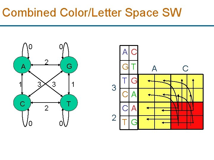
Combined Color/Letter Space SW 0 0 2 A 1 3 C GT G 3 1 3 T 2 0 A C 0 T G CA CA 2 T G A C
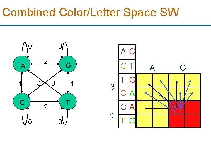
Combined Color/Letter Space SW 0 0 2 A 1 3 C GT G 3 1 3 T 2 0 A C 0 T G CA CA 2 T G A C
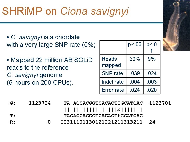
SHRi. MP on Ciona savignyi • C. savignyi is a chordate with a very large SNP rate (5%) • Mapped 22 million AB SOLi. D reads to the reference C. savignyi genome (6 hours on 200 CPUs). G: 1123724 T: R: 0 p<. 05 p<. 0 1 Reads mapped 20% 9% SNP rate . 039 . 024 Indel rate . 004 . 003 Error rate . 024 . 020 TA-ACCACGGTCACACTTGCATCAC || ||||| |||X||||||| TACACCACGGTCAGACTt. GCATCAC T 0311101130121221211313211 1123701 24
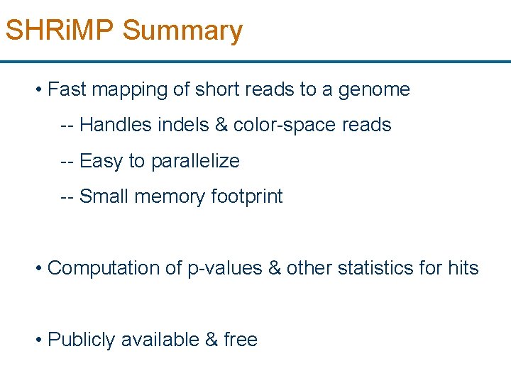
SHRi. MP Summary • Fast mapping of short reads to a genome -- Handles indels & color-space reads -- Easy to parallelize -- Small memory footprint • Computation of p-values & other statistics for hits • Publicly available & free
Acknowledgments Stephen Rumble Phil Lacroute Anton Valouev Arend Sidow Uof. T Stanford http: //compbio. cs. toronto. edu/shrimp FUNDING: NSERC, CFI, NIH
Acknowledgments Stephen Rumble Phil Lacroute Anton Valouev Arend Sidow Uof. T Stanford http: //compbio. cs. toronto. edu/shrimp FUNDING: NSERC, CFI, NIH
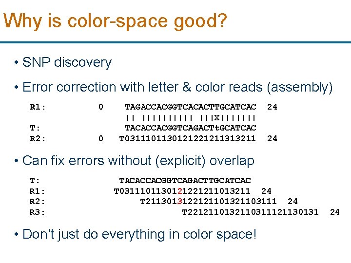
Why is color-space good? • SNP discovery • Error correction with letter & color reads (assembly) R 1: 0 T: R 2: 0 TAGACCACGGTCACACTTGCATCAC || ||||| |||X||||||| TACACCACGGTCAGACTt. GCATCAC T 0311101130121221211313211 24 24 • Can fix errors without (explicit) overlap T: R 1: R 2: R 3: TACACCACGGTCAGACTTGCATCAC T 0311101130121221211013211 24 T 2113013122121101321103111 24 T 2212110132110311121130131 • Don’t just do everything in color space! 24
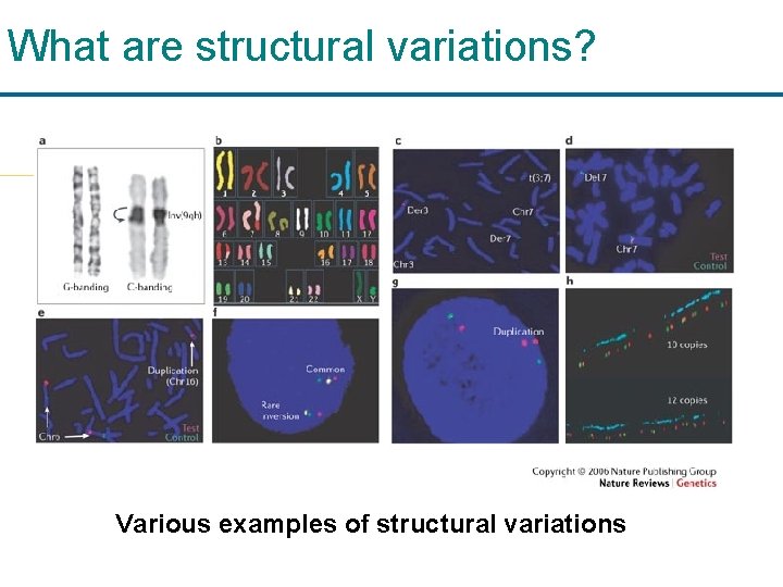
What are structural variations? Various examples of structural variations
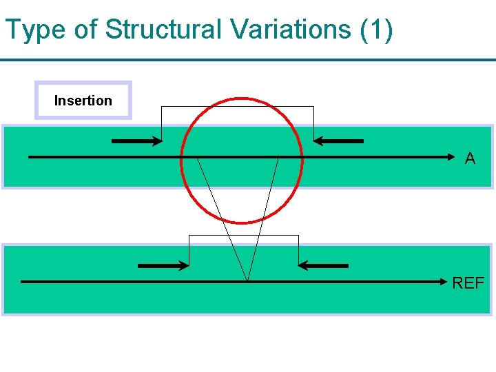
Type of Structural Variations (1) Insertion A REF
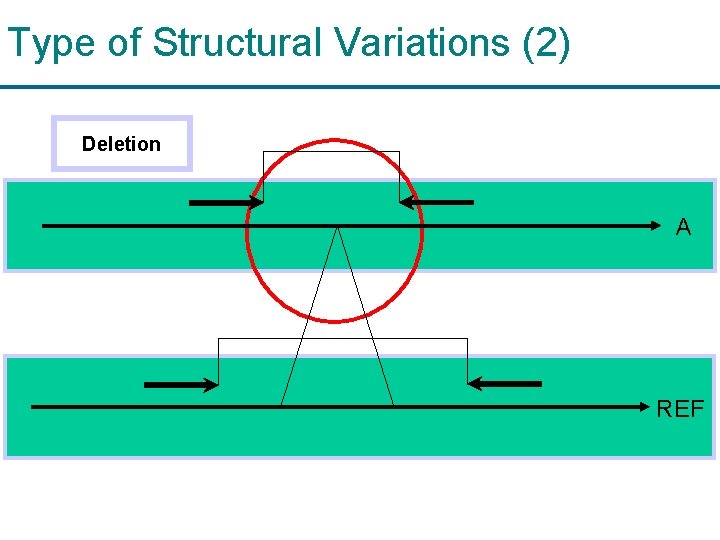
Type of Structural Variations (2) Deletion A REF
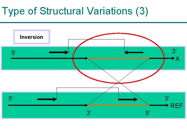
Type of Structural Variations (3) Inversion 3’ A 5’ 5’ 3’ REF 3’ 5’
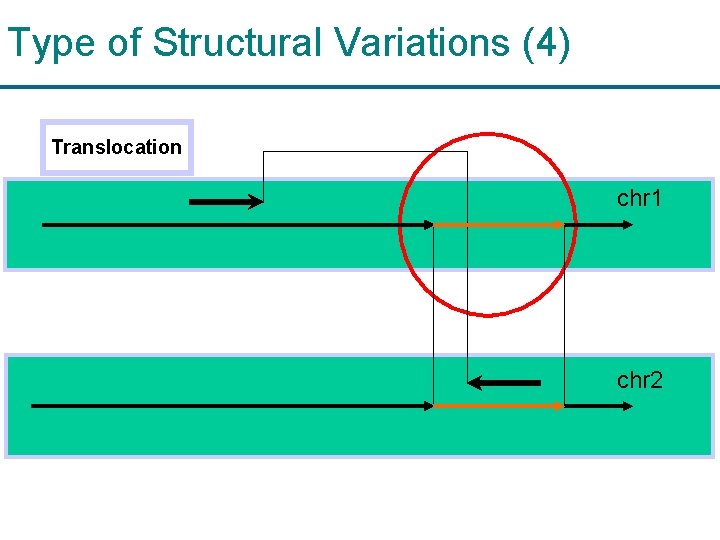
Type of Structural Variations (4) Translocation chr 1 chr 2
Clone-end Sequencing Approaches 1. “Fine-scale structural variation of the human genome” [Tuzun et al, 2005] • Mapping matepairs onto the reference genome • If mappings of matepairs are not consistent, then there exist structural variations. 2. “Paired-End mappings Reveals Extensive Structural Variation in the Human Genome” [Korbel et al, 2007] • Proposed high-throughput and massive paired end mapping technique • Detailed types of structural variations
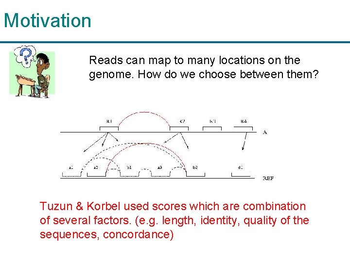
Motivation Reads can map to many locations on the genome. How do we choose between them? Tuzun & Korbel used scores which are combination of several factors. (e. g. length, identity, quality of the sequences, concordance)
Probabilistic Framework (1) We play with p(Y) to describe our probabilistic framework p(Y): distribution of mapped distances of “uniquely mapped” matepairs of various sizes
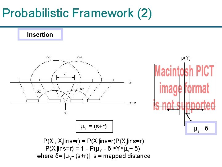
Probabilistic Framework (2) Insertion p(Y) μY = (s+r) P(Xi, Xj|ins=r) = P(Xi|ins=r)P(Xj|ins=r) P(Xi|ins=r) = 1 - P(μY - δ ≤Y≤μy+ δ) where δ= |μY- (s+r)|, s = mapped distance μy - δ
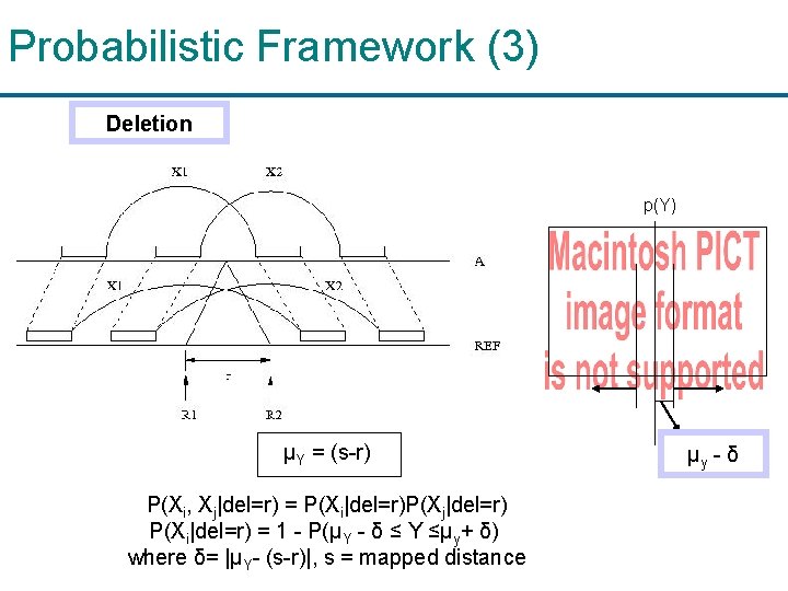
Probabilistic Framework (3) Deletion p(Y) μY = (s-r) P(Xi, Xj|del=r) = P(Xi|del=r)P(Xj|del=r) P(Xi|del=r) = 1 - P(μY - δ ≤ Y ≤μy+ δ) where δ= |μY- (s-r)|, s = mapped distance μy - δ

Probabilistic Framework (4) Inversion p(|Y 1 -Y 2|) μ|Y 1 -Y 2|-δ c - d = s(X 1) - s(X 2) P(Xi, Xj|inv) = 1 - P(μ|Y 1 -Y 2| - δ ≤|Y 1 -Y 2|≤μ|Y 1 -Y 2| + δ) where δ= |μ|Y 1 -Y 2| – (c – d)|
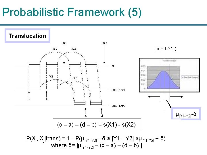
Probabilistic Framework (5) Translocation p(|Y 1 -Y 2|) μ|Y 1 -Y 2|-δ (c – a) – (d – b) = s(X 1) - s(X 2) P(Xi, Xj|trans) = 1 - P(μ|Y 1 -Y 2| - δ ≤ |Y 1 - Y 2| ≤μ|Y 1 -Y 2| + δ) where δ= |μ|Y 1 -Y 2| – (c – a) – (d – b) |
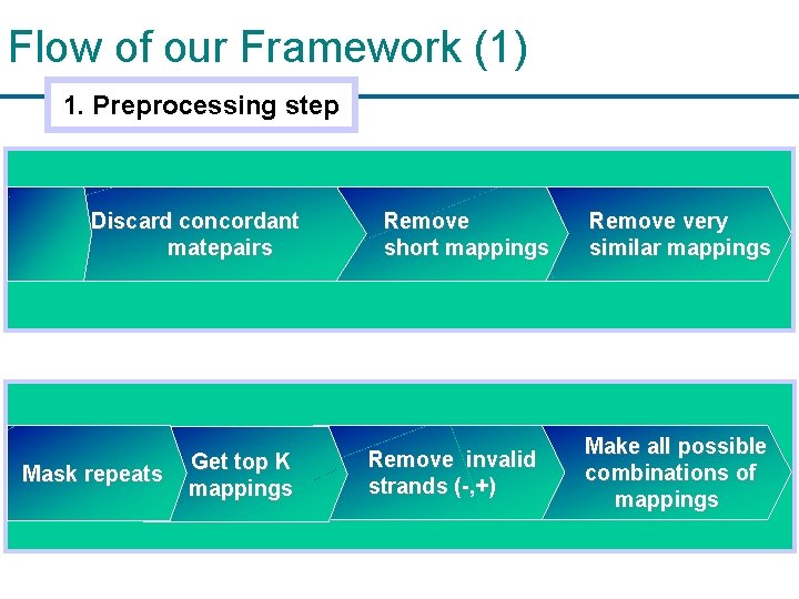
Flow of our Framework (1) 1. Preprocessing step Discard concordant matepairs Mask repeats Get top K mappings Remove short mappings Remove invalid strands (-, +) Remove very similar mappings Make all possible combinations of mappings
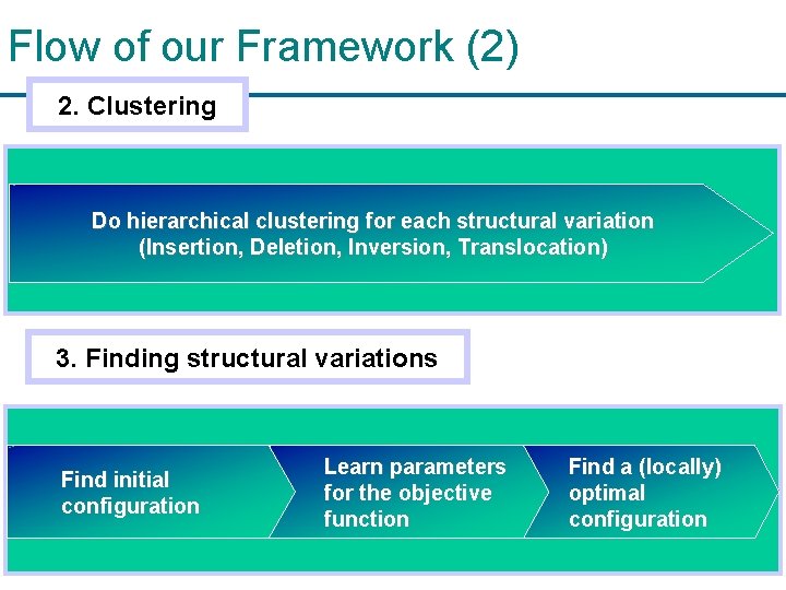
Flow of our Framework (2) 2. Clustering Do hierarchical clustering for each structural variation (Insertion, Deletion, Inversion, Translocation) 3. Finding structural variations Find initial configuration Learn parameters for the objective function Find a (locally) optimal configuration
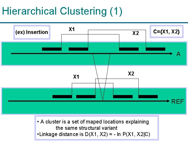
Hierarchical Clustering (1) (ex) Insertion X 1 X 2 C={X 1, X 2} A X 1 X 2 REF • A cluster is a set of maped locations explaining the same structural variant • Linkage distance is D(X 1, X 2) = - ln P(X 1, X 2|C)
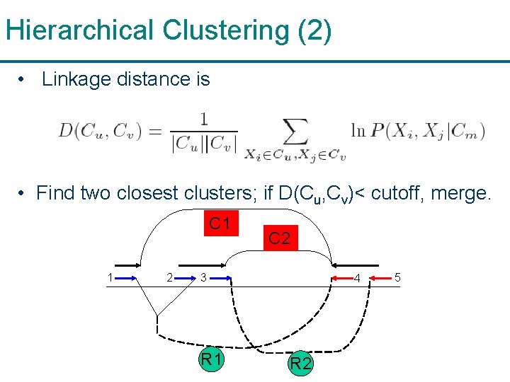
Hierarchical Clustering (2) • Linkage distance is • Find two closest clusters; if D(Cu, Cv)< cutoff, merge. C 1 1 2 C 2 3 R 1 4 R 2 5
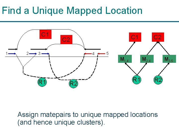
Find a Unique Mapped Location C 1 1 2 C 1 C 2 3 4 5 M 1, 4 R 1 R 2 C 2 M 2, 4 R 1 M 3, 5 R 2 Assign matepairs to unique mapped locations (and hence unique clusters).
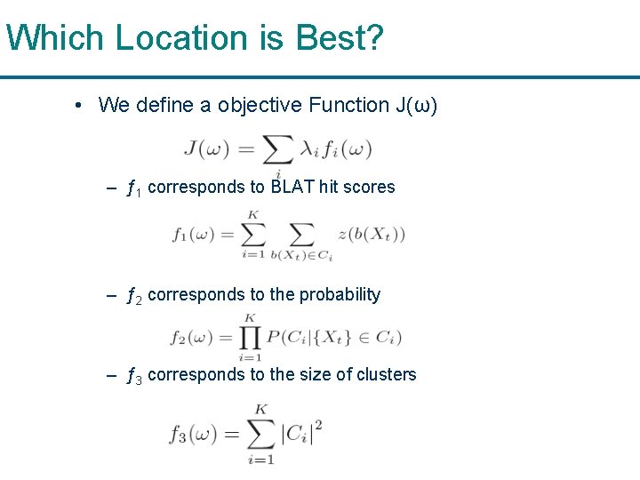
Which Location is Best? • We define a objective Function J(ω) – ƒ 1 corresponds to BLAT hit scores – ƒ 2 corresponds to the probability – ƒ 3 corresponds to the size of clusters
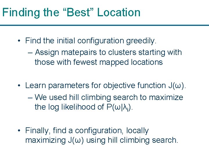
Finding the “Best” Location • Find the initial configuration greedily. – Assign matepairs to clusters starting with those with fewest mapped locations • Learn parameters for objective function J(ω). – We used hill climbing search to maximize the log likelihood of P(ω|λi). • Finally, find a configuration, locally maximizing J(ω) using hill climbing search.
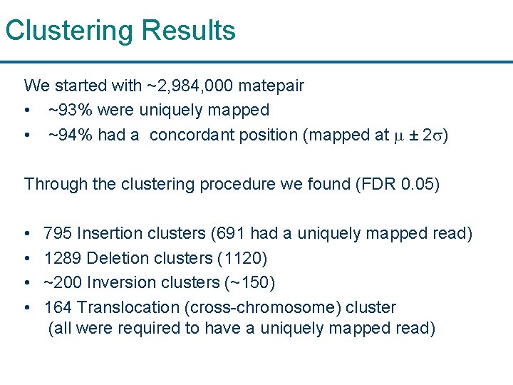
Clustering Results We started with ~2, 984, 000 matepair • ~93% were uniquely mapped • ~94% had a concordant position (mapped at ± 2 ) Through the clustering procedure we found (FDR 0. 05) • • 795 Insertion clusters (691 had a uniquely mapped read) 1289 Deletion clusters (1120) ~200 Inversion clusters (~150) 164 Translocation (cross-chromosome) cluster (all were required to have a uniquely mapped read)
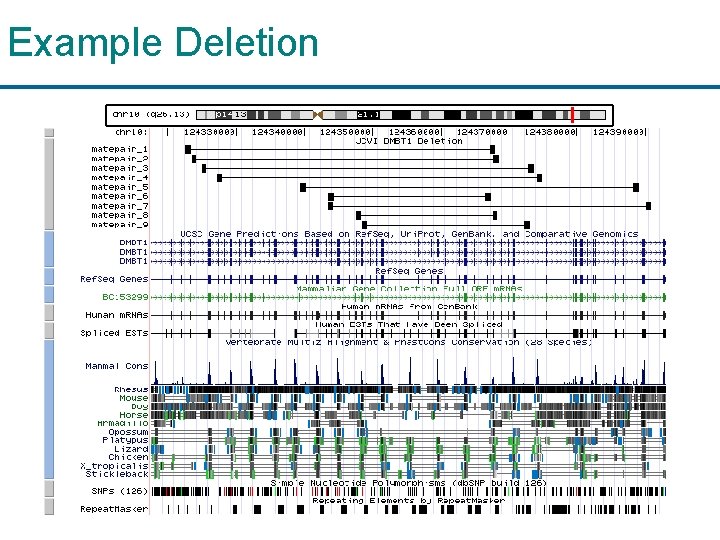
Example Deletion
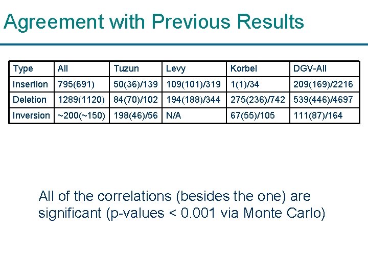
Agreement with Previous Results Type All Tuzun Levy Insertion 795(691) 50(36)/139 109(101)/319 Deletion 1289(1120) 84(70)/102 194(188)/344 Inversion ~200(~150) 198(46)/56 N/A Korbel DGV-All 1(1)/34 209(169)/2216 275(236)/742 539(446)/4697 67(55)/105 111(87)/164 All of the correlations (besides the one) are We have compared significant (p-values < 0. 001 via Monte Carlo)
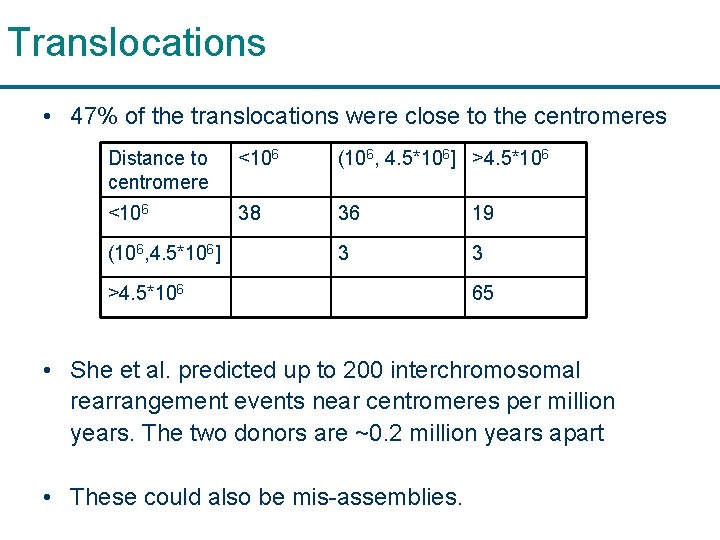
Translocations • 47% of the translocations were close to the centromeres Distance to centromere <106 (106, 4. 5*106] >4. 5*106 <106 38 36 19 3 3 (106, 4. 5*106] >4. 5*106 65 • She et al. predicted up to 200 interchromosomal rearrangement events near centromeres per million years. The two donors are ~0. 2 million years apart • These could also be mis-assemblies.
Summary (Structural Variation) • Introduced a probabilistic framework for finding structural variants that does not rely on ab initio mapping of matepairs to genomic positions. • Isolated hundreds of insertions, deletions, and inversions between the reference public human genome and the JCVI donor. • These results show statistically significant correlation with previous variation studies • About 2/3 of the structural variants we isolate is not found in the Database of Genomic Variants
What about Copy Number Variants? • Copy Number Variants are the result of duplications and deletions of large genomic segments • Currently mainly found using microarray technology (ROMA, CGH) • There is no algorithm for CNV finding with short reads (? ) • Goal: predict the number of times a certain segment appears in the genome
A Little Bit of Math Let C = #reads / length of genome Let i be a read Let xi be # of times it was sampled. Assembled genome should contain every read about xi / C times. For example, let C = 3, xi = 7
More formally Let n = number of reads, N = length of the genome • The probability Pi that the read i was sampled xi times given that it appears in the genome gi times is • We want to maximize the likelihood that all of the reads were sampled from the genome: • However there is an additional constraint
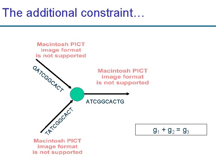
The additional constraint… GA TC GG CA CT TA TC G G C AC T ATCGGCACTG g 1 + g 2 = g 3
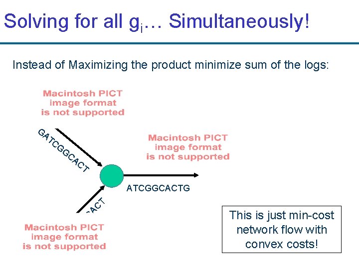
Solving for all gi… Simultaneously! Instead of Maximizing the product minimize sum of the logs: GA TC GG CA CT TA TC G G C AC T ATCGGCACTG This is just min-cost network flow with convex costs!
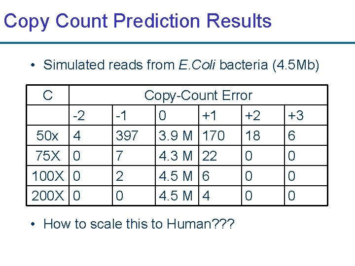
Copy Count Prediction Results • Simulated reads from E. Coli bacteria (4. 5 Mb) C -2 50 x 4 75 X 0 100 X 0 200 X 0 Copy-Count Error -1 0 +1 +2 397 3. 9 M 170 18 7 4. 3 M 22 0 2 4. 5 M 6 0 0 4. 5 M 4 0 • How to scale this to Human? ? ? +3 6 0 0 0
Discovering Variation • SHRi. MP -- SHort Read Mapping Package – Computes p-values & other statistics – Specialized Color-space alignment • Algorithm for Structural Variation Discovery – Will it scale to short reads? • A model for Copy Count Prediction – Works well with reads from E. coli, but how to scale to Human?
- Slides: 73