High Performance Parallel Stochastic Gradient Descent IN SHARED

High Performance Parallel Stochastic Gradient Descent IN SHARED MEMORY Scott Sallinen, 2 Nadathur Satish, 2 Mikhail Smelyanskiy, 2 Samantika Sury, 3 Christopher Ré 1, 2 1 University of British Columbia, 2 Intel Corporation, 3 Stanford University

Overview of Regression and Stochastic gradient descent Overview of Regression & SGD Parallelizing SGD Experimental Results Comparison to State of the Art

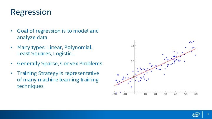
Regression • Goal of regression is to model and analyze data • Many types: Linear, Polynomial, Least Squares, Logistic… • Generally Sparse, Convex Problems • Training Strategy is representative of many machine learning training techniques 3

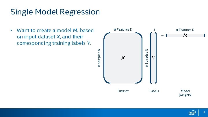
Single Model Regression • Want to create a model M, based on input dataset X, and their corresponding training labels Y. 1 # Features D X Dataset # Samples N 1 # Features D M Y Labels Model (weights) 4

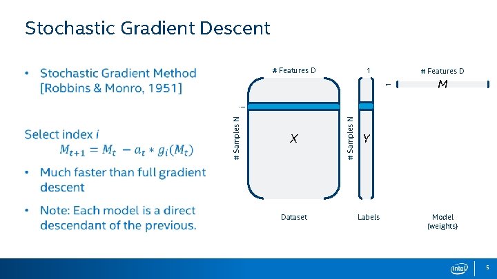
Stochastic Gradient Descent 1 # Features D M X Dataset # Samples N i 1 # Features D Y Labels Model (weights) 5

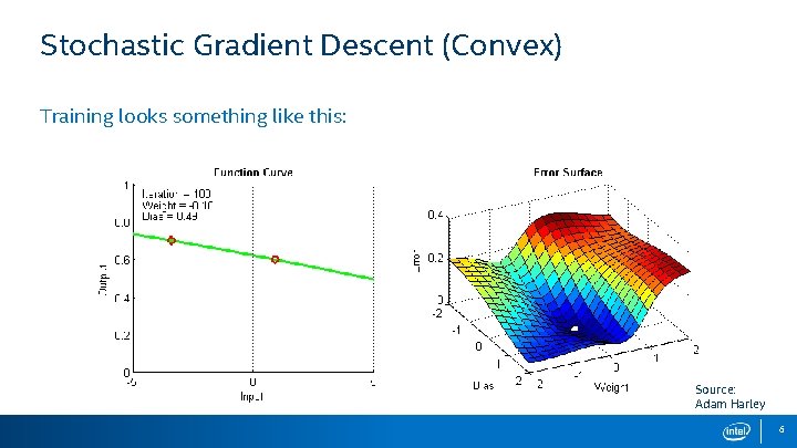
Stochastic Gradient Descent (Convex) Training looks something like this: Source: Adam Harley 6

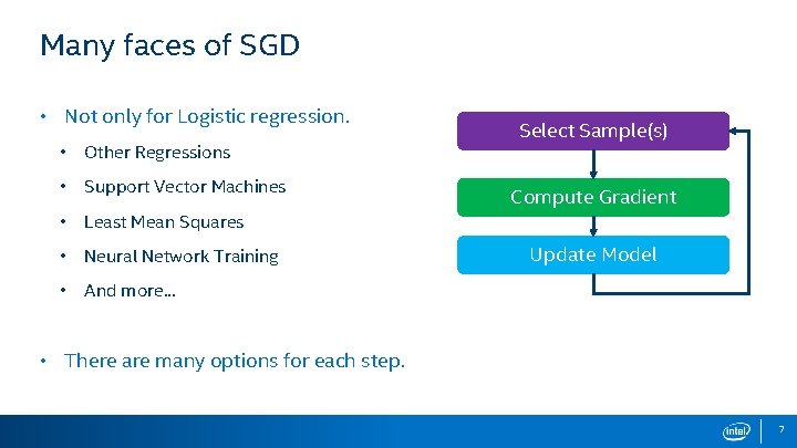
Many faces of SGD • Not only for Logistic regression. • Other Regressions • Support Vector Machines • Least Mean Squares • Neural Network Training • And more. . . Select Sample(s) Compute Gradient Update Model • There are many options for each step. 7

Parallelizing Stochastic Gradient Descent Overview of Regression & SGD Parallelizing SGD Experimental Results Comparison to State of the Art

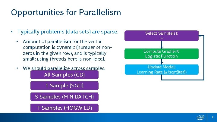
Opportunities for Parallelism • Typically problems (data sets) are sparse. • • Select Sample(s): ~ Amount of parallelism for the vector computation is dynamic (number of nonzeros in the given row), and is typically small: using threads here is non-ideal. We should parallelize across samples. All Samples (GD) Compute Gradient: Logistic Function 1 Sample (SGD) S Samples (MINIBATCH) T Samples (HOGWILD) 9

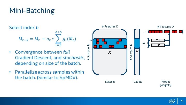
Mini-Batching 1 # Features D M 1 # Features D X Dataset S # Samples N b T 1 T 2 Y Labels Model (weights) 10

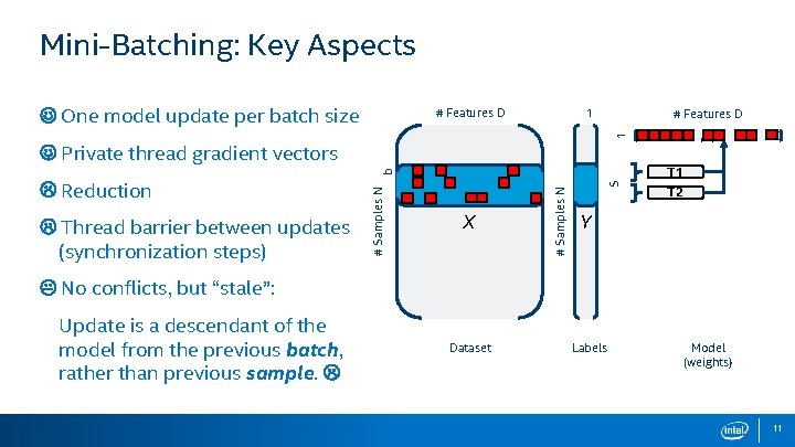
Mini-Batching: Key Aspects One model update per batch size 1 # Features D M 1 # Features D Private thread gradient vectors Thread barrier between updates (synchronization steps) X S # Samples N Reduction # Samples N b T 1 T 2 Y No conflicts, but “stale”: Update is a descendant of the model from the previous batch, rather than previous sample. Dataset Labels Model (weights) 11

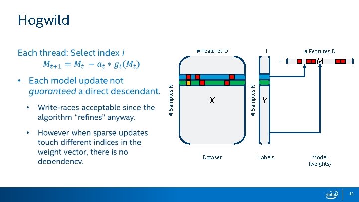
Hogwild 1 # Features D X Dataset # Samples N 1 # Features D M Y Labels Model (weights) 12

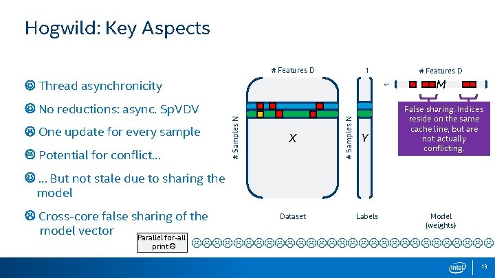
Hogwild: Key Aspects # Features D 1 Potential for conflict… X # Samples N One update for every sample # Samples N No reductions: async. Sp. VDV 1 Thread asynchronicity # Features D Y M False sharing: Indices reside on the same cache line, but are not actually conflicting. … But not stale due to sharing the model Dataset Labels Model Cross-core false sharing of the (weights) model vector Parallel for-all print 13

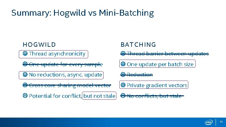
Summary: Hogwild vs Mini-Batching HOGWILD BATCHING Thread asynchronicity Thread barrier between updates One update for every sample One update per batch size No reductions, async. update Reduction Cross core sharing model vector Private gradient vectors Potential for conflict, but not stale No conflicts, but stale 14

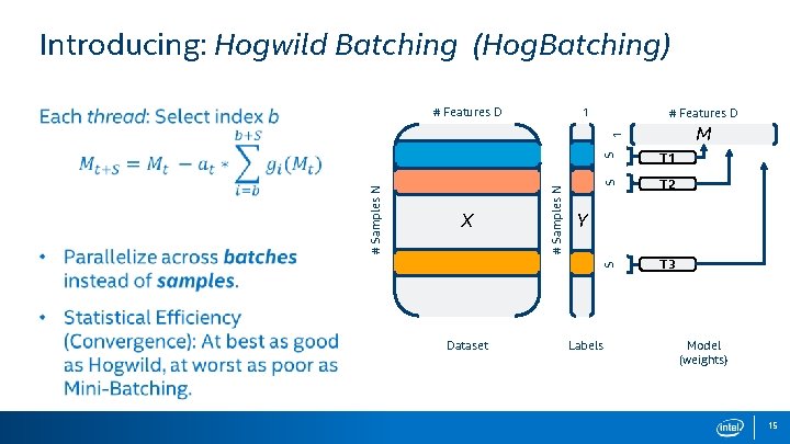
Introducing: Hogwild Batching (Hog. Batching) 1 # Features D M Dataset S T 1 S T 2 S X # Samples N 1 # Features D T 3 Y Labels Model (weights) 15

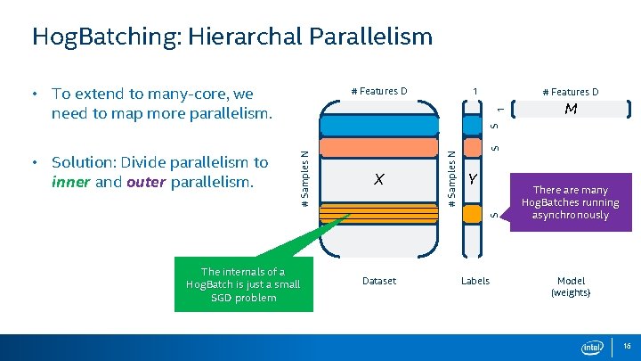
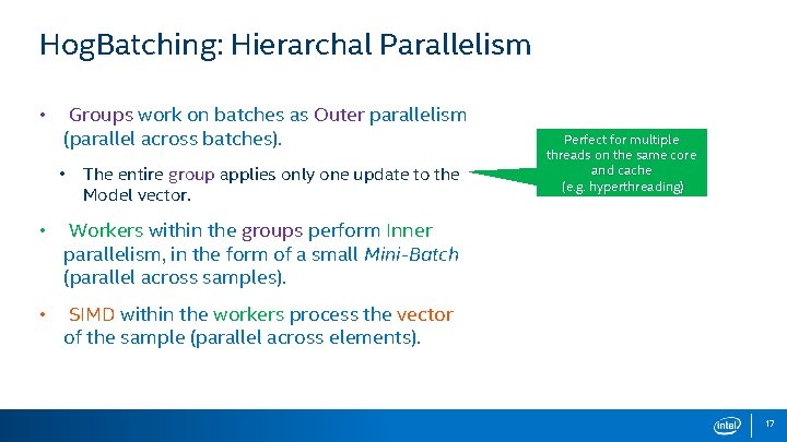
Hog. Batching: Hierarchal Parallelism • To extend to many-core, we need to map more parallelism. 1 M S S 1 # Features D Y S X # Samples N • Solution: Divide parallelism to inner and outer parallelism. # Features D The internals of a Hog. Batch is just a small SGD problem Dataset Labels There are many Hog. Batches running asynchronously Model (weights) 16

Hog. Batching: Hierarchal Parallelism • Groups work on batches as Outer parallelism (parallel across batches). • The entire group applies only one update to the Model vector. • Workers within the groups perform Inner parallelism, in the form of a small Mini-Batch (parallel across samples). • SIMD within the workers process the vector of the sample (parallel across elements). Perfect for multiple threads on the same core and cache (e. g. hyperthreading) 17

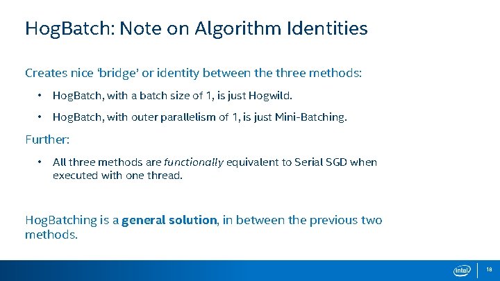
Hog. Batch: Note on Algorithm Identities Creates nice ‘bridge’ or identity between the three methods: • Hog. Batch, with a batch size of 1, is just Hogwild. • Hog. Batch, with outer parallelism of 1, is just Mini-Batching. Further: • All three methods are functionally equivalent to Serial SGD when executed with one thread. Hog. Batching is a general solution, in between the previous two methods. 18

Experimental Results Overview of Regression & SGD Parallelizing SGD Experimental Results Comparison to State of the Art

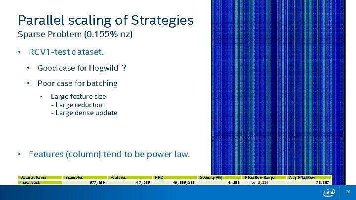
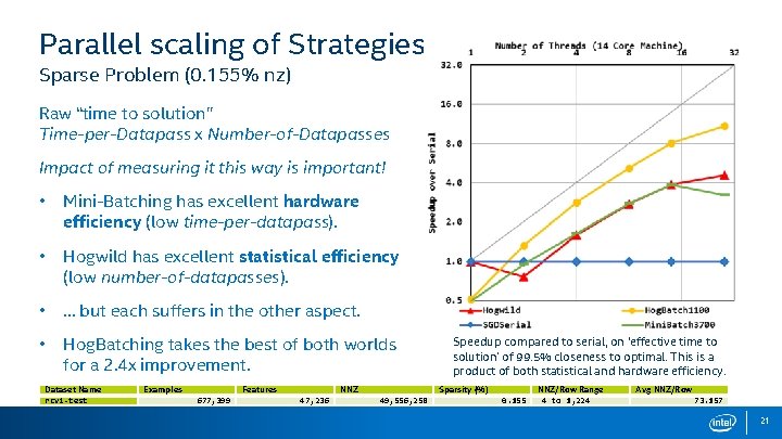
Parallel scaling of Strategies Sparse Problem (0. 155% nz) • RCV 1 -test dataset. • Good case for Hogwild ? • Poor case for batching • Large feature size - Large reduction - Large dense update • Features (column) tend to be power law. Dataset Name rcv 1 -test Examples Features 677, 399 NNZ 47, 236 Sparsity (%) 49, 556, 258 0. 155 NNZ/Row Range 4 to 1, 224 Avg NNZ/Row 73. 157 20

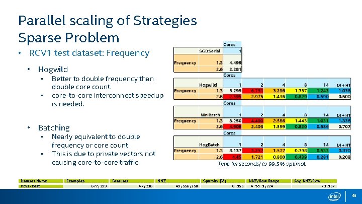
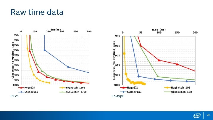
Parallel scaling of Strategies Sparse Problem (0. 155% nz) Raw “time to solution” Time-per-Datapass x Number-of-Datapasses Impact of measuring it this way is important! • Mini-Batching has excellent hardware efficiency (low time-per-datapass). • Hogwild has excellent statistical efficiency (low number-of-datapasses). • … but each suffers in the other aspect. • Hog. Batching takes the best of both worlds for a 2. 4 x improvement. Dataset Name rcv 1 -test Examples Features 677, 399 NNZ 47, 236 Speedup compared to serial, on ‘effective time to solution’ of 99. 5% closeness to optimal. This is a product of both statistical and hardware efficiency. Sparsity (%) 49, 556, 258 0. 155 NNZ/Row Range 4 to 1, 224 Avg NNZ/Row 73. 157 21

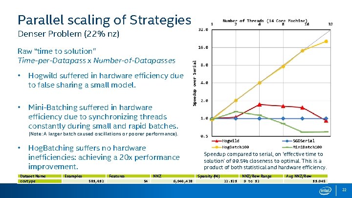
Parallel scaling of Strategies Denser Problem (22% nz) Raw “time to solution” Time-per-Datapass x Number-of-Datapasses • Hogwild suffered in hardware efficiency due to false sharing a small model. • Mini-Batching suffered in hardware efficiency due to synchronizing threads constantly during small and rapid batches. (Note: A larger batch caused oscillations or poorer performance). • Hog. Batching suffers no hardware inefficiencies: achieving a 20 x performance improvement. Dataset Name covtype Examples Features 581, 012 NNZ 54 Speedup compared to serial, on ‘effective time to solution’ of 99. 5% closeness to optimal. This is a product of both statistical and hardware efficiency. Sparsity (%) 6, 940, 438 22. 121 NNZ/Row Range 9 to 12 Avg NNZ/Row 11. 945 22

Comparison to state-of-the-art Overview of Regression & SGD Parallelizing SGD Experimental Results Comparison to State of the Art

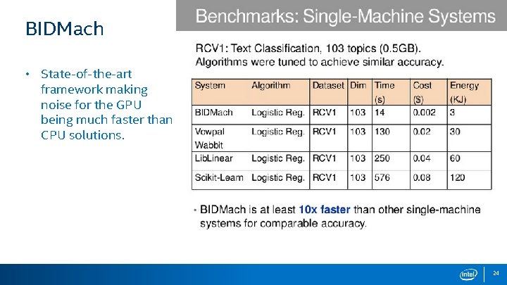
BIDMach • State-of-the-art framework making noise for the GPU being much faster than CPU solutions. 24

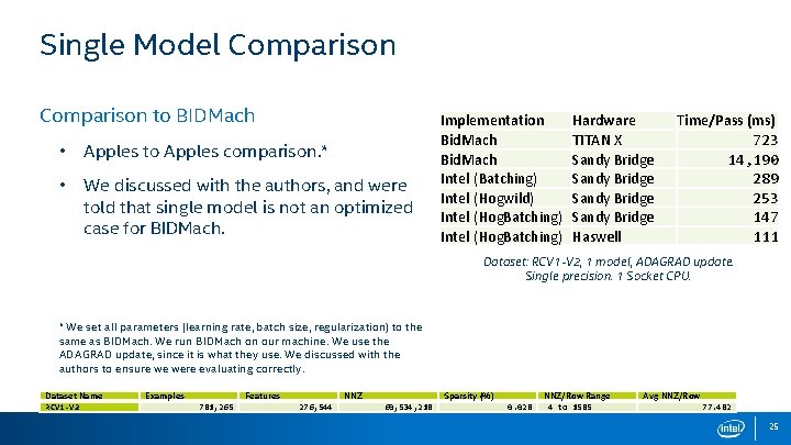
Single Model Comparison to BIDMach • Apples to Apples comparison. * • We discussed with the authors, and were told that single model is not an optimized case for BIDMach. Implementation Bid. Mach Intel (Batching) Intel (Hogwild) Intel (Hog. Batching) Hardware TITAN X Sandy Bridge Haswell Time/Pass (ms) 723 14, 190 289 253 147 111 Dataset: RCV 1 -V 2, 1 model, ADAGRAD update. Single precision. 1 Socket CPU. * We set all parameters (learning rate, batch size, regularization) to the same as BIDMach. We run BIDMach on our machine. We use the ADAGRAD update, since it is what they use. We discussed with the authors to ensure we were evaluating correctly. Dataset Name RCV 1 -V 2 Examples Features 781, 265 NNZ 276, 544 Sparsity (%) 60, 534, 218 0. 028 NNZ/Row Range 4 to 1585 Avg NNZ/Row 77. 482 25

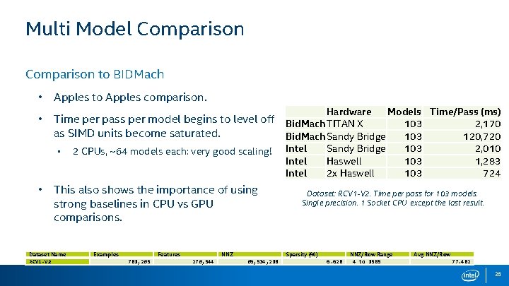
Multi Model Comparison to BIDMach • Apples to Apples comparison. • Time per pass per model begins to level off Bid. Mach TITAN X as SIMD units become saturated. Bid. Mach Sandy Bridge Hardware • • 2 CPUs, ~64 models each: very good scaling! This also shows the importance of using strong baselines in CPU vs GPU comparisons. Dataset Name RCV 1 -V 2 Examples Features 781, 265 NNZ 276, 544 Intel Models Time/Pass (ms) 103 2, 170 103 120, 720 Sandy Bridge 103 2, 010 Haswell 103 1, 283 2 x Haswell 103 724 Dataset: RCV 1 -V 2. Time per pass for 103 models. Single precision. 1 Socket CPU except the last result. Sparsity (%) 60, 534, 218 0. 028 NNZ/Row Range 4 to 1585 Avg NNZ/Row 77. 482 26

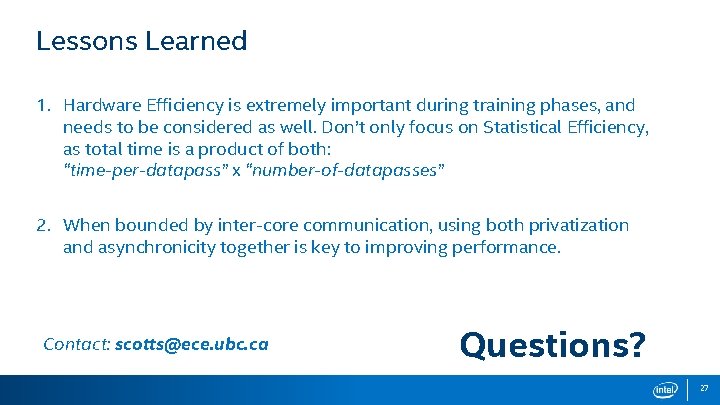
Lessons Learned 1. Hardware Efficiency is extremely important during training phases, and needs to be considered as well. Don’t only focus on Statistical Efficiency, as total time is a product of both: “time-per-datapass” x “number-of-datapasses” 2. When bounded by inter-core communication, using both privatization and asynchronicity together is key to improving performance. Contact: scotts@ece. ubc. ca Questions? 27

Backup slides

Overview of Regression & SGD Parallelizing SGD Multi Model Regression Experimental Results Multi Model Regression Comparison to State of the Art

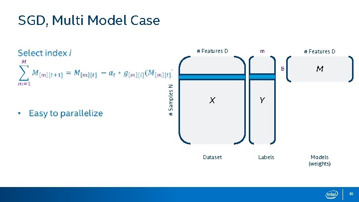
SGD, Multi Model Case m # Features D # Samples N m # Features D X Dataset M Y Labels Models (weights) 30

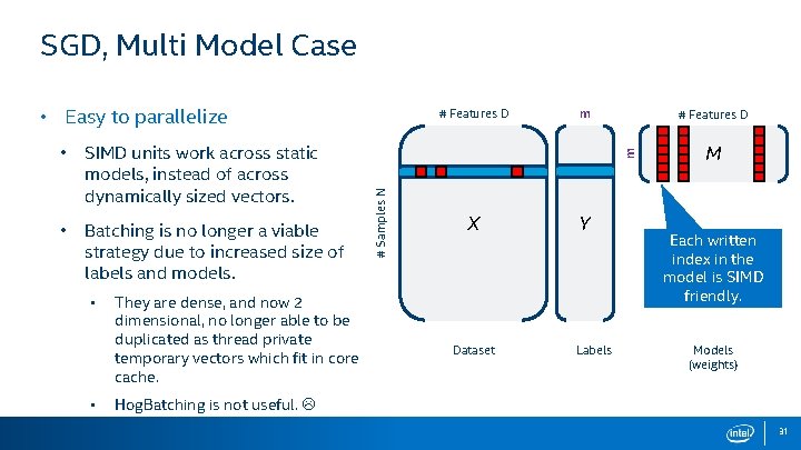
SGD, Multi Model Case • Easy to parallelize • Batching is no longer a viable strategy due to increased size of labels and models. • • They are dense, and now 2 dimensional, no longer able to be duplicated as thread private temporary vectors which fit in core cache. m # Features D m SIMD units work across static models, instead of across dynamically sized vectors. # Samples N • # Features D X Dataset Y Labels M Each written index in the model is SIMD friendly. Models (weights) Hog. Batching is not useful. 31

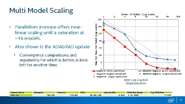
Multi Model Scaling • Parallelism increase offers nearlinear scaling until a saturation at ~16 models. • Also shown is the ADAGRAD update. • Convergence comparisons and arguments for which is better, is best left for another time. Note: Log-Log Axis. Single precision. Dataset Name RCV 1 -V 2 Examples Features 781, 265 NNZ 276, 544 Sparsity (%) 60, 534, 218 0. 028 NNZ/Row Range 4 to 1585 Avg NNZ/Row 77. 482 32

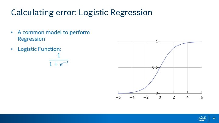
Calculating error: Logistic Regression 33

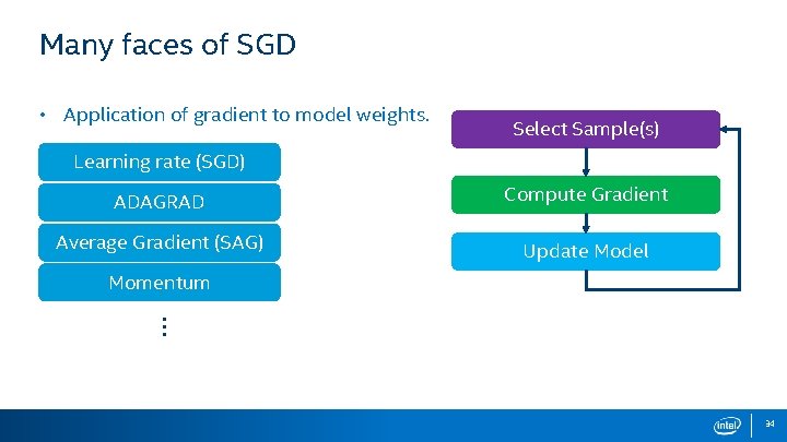
Many faces of SGD • Application of gradient to model weights. Select Sample(s) Learning rate (SGD) ADAGRAD Compute Gradient Average Gradient (SAG) Update Model Momentum … 34

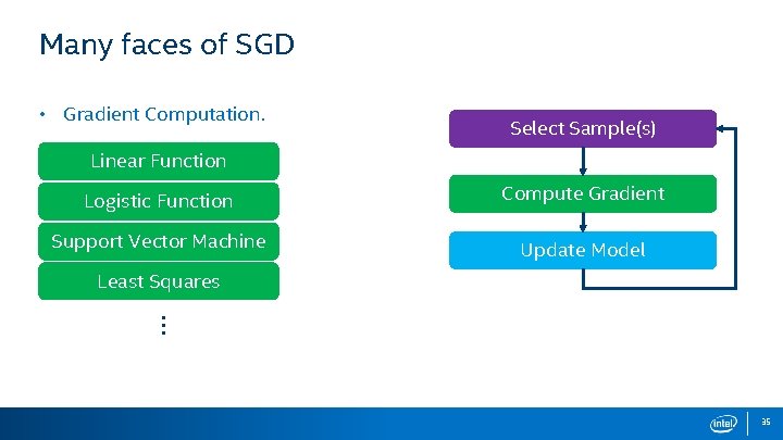
Many faces of SGD • Gradient Computation. Select Sample(s) Linear Function Logistic Function Compute Gradient Support Vector Machine Update Model Least Squares … 35

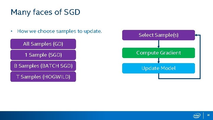
Many faces of SGD • How we choose samples to update. Select Sample(s) All Samples (GD) 1 Sample (SGD) Compute Gradient B Samples (BATCH SGD) Update Model T Samples (HOGWILD) 36

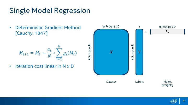
Single Model Regression 1 # Features D X Dataset # Samples N 1 # Features D M Y Labels Model (weights) 37

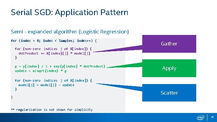
Serial SGD: Application Pattern Semi - expanded algorithm (Logistic Regression) for (index = 0; index < Samples; index++) { for (non-zero indices j of X[index]) { dot. Product += X[index][j] * model[j] } g = y[index ] / 1 + exp(y[index] * dot. Product) update = a/sqrt(index) * g for (non-zero indices j of X[index]) { model[j] = model[j] – update } } Gather Apply Scatter ** regularization is not shown for simplicity 38

Serial SGD: Dependency Pattern Expanded Logistic Regression 1 # Features D g = y[index] / 1 + exp(y[index] * dot. Prod) update = a/sqrt(index) * g X # Samples N for (non-zero indices j of X[index]) { dot. Prod += X[index][j] * model[j] } # Samples N for (index = 0; index < Samples; index++) { M Y for (non-zero indices j of X[index]) { model[j] = model[j] – update } } Update only touches sparse indices in the vector Dataset Labels Model (weights) ** regularization is not shown for simplicity 39

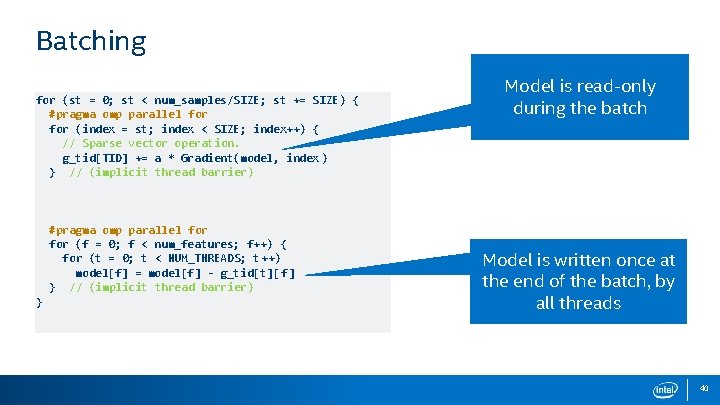
Batching for (st = 0; st < num_samples/SIZE; st += SIZE) { #pragma omp parallel for (index = st; index < SIZE; index++) { // Sparse vector operation. g_tid[TID] += a * Gradient(model, index ) } // (implicit thread barrier) #pragma omp parallel for (f = 0; f < num_features; f++) { for (t = 0; t < NUM_THREADS; t++) model[f] = model[f] - g_tid[t][ f] } // (implicit thread barrier) } Model is read-only during the batch Model is written once at the end of the batch, by all threads 40

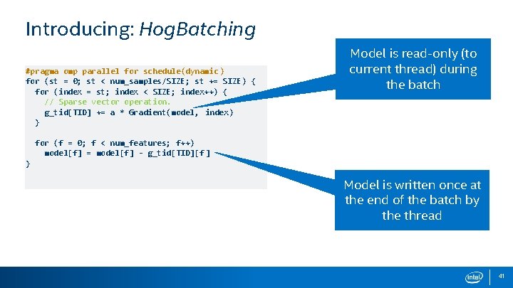
Introducing: Hog. Batching #pragma omp parallel for schedule(dynamic ) for (st = 0; st < num_samples/SIZE; st += SIZE) { for (index = st; index < SIZE; index++) { // Sparse vector operation. g_tid[TID] += a * Gradient(model, index) } Model is read-only (to current thread) during the batch for (f = 0; f < num_features; f++) model[f] = model[f] - g_tid[TID][f ] } Model is written once at the end of the batch by the thread 41

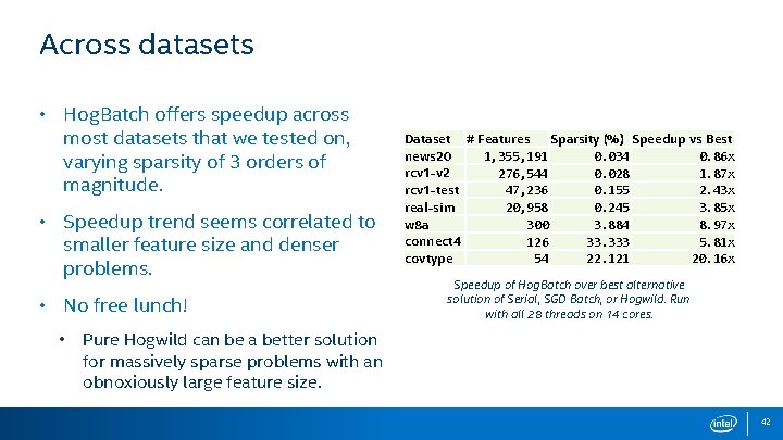
Across datasets • Hog. Batch offers speedup across most datasets that we tested on, varying sparsity of 3 orders of magnitude. • Speedup trend seems correlated to smaller feature size and denser problems. • No free lunch! • Dataset # Features Sparsity (%) Speedup vs Best news 20 1, 355, 191 0. 034 0. 86 x rcv 1 -v 2 276, 544 0. 028 1. 87 x rcv 1 -test 47, 236 0. 155 2. 43 x real-sim 20, 958 0. 245 3. 85 x w 8 a 300 3. 884 8. 97 x connect 4 126 33. 333 5. 81 x covtype 54 22. 121 20. 16 x Speedup of Hog. Batch over best alternative solution of Serial, SGD Batch, or Hogwild. Run with all 28 threads on 14 cores. Pure Hogwild can be a better solution for massively sparse problems with an obnoxiously large feature size. 42

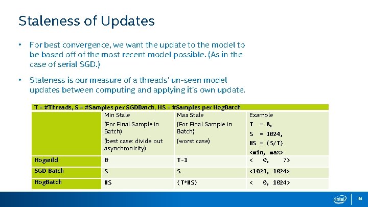
Staleness of Updates • For best convergence, we want the update to the model to be based off of the most recent model possible. (As in the case of serial SGD. ) • Staleness is our measure of a threads’ un-seen model updates between computing and applying it’s own update. T = #Threads, S = #Samples per SGDBatch, HS = #Samples per Hog. Batch Min Stale Max Stale Example (For Final Sample in Batch) T = 8, (best case: divide out asynchronicity) (worst case) S = 1024, HS = (S/T) Hogwild 0 T-1 <min, max> < 0, 7> SGD Batch S S <1024, 1024> Hog. Batch HS (T*HS) < 0, 1024> 43

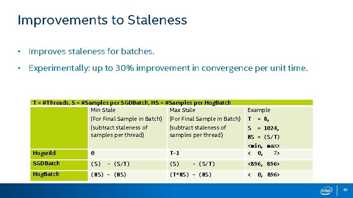
Improvements to Staleness • Improves staleness for batches. • Experimentally: up to 30% improvement in convergence per unit time. T = #Threads, S = #Samples per SGDBatch, HS = #Samples per Hog. Batch Min Stale Max Stale Example (For Final Sample in Batch) T = 8, (subtract staleness of samples per thread) S = 1024, Hogwild 0 SGDBatch (S) Hog. Batch (HS) – (HS) <min, max> < 0, 7> T-1 - (S/T) (S) HS = (S/T) - (S/T) (T*HS) – (HS) <896, 896> < 0, 896> 44

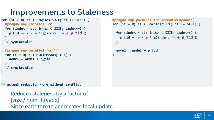
Improvements to Staleness for (st = 0; st < Samples/SIZE; st += SIZE) { #pragma omp parallel for (index = st; index < SIZE; index++) { p_tid += w – a * g(index, [w + p_tid ]) } // synchronize #pragma omp parallel for ** for (t = 0; t < num. Threads; t++) { model = model + p_tid } // synchronize #pragma omp parallel for schedule(dynamic) for (st = 0; st < Samples/SIZE; st += SIZE) { for (index = st; index < SIZE; index++) { p_tid += w – a * g(index, [w + p_tid ]) } model = model + p_tid } } ** actual reduction done without conflict Reduces staleness by a factor of [size / num. Threads] Since each thread aggregates local update. 45

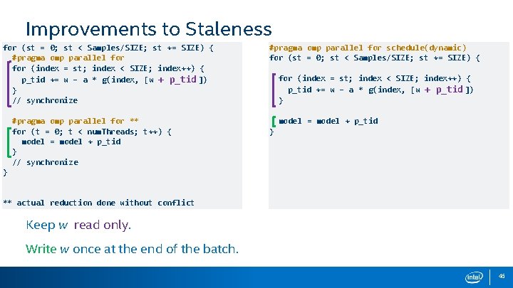
Improvements to Staleness for (st = 0; st < Samples/SIZE; st += SIZE) { #pragma omp parallel for (index = st; index < SIZE; index++) { p_tid += w – a * g(index, [w + p_tid ]) } // synchronize #pragma omp parallel for ** for (t = 0; t < num. Threads; t++) { model = model + p_tid } // synchronize #pragma omp parallel for schedule(dynamic) for (st = 0; st < Samples/SIZE; st += SIZE) { for (index = st; index < SIZE; index++) { p_tid += w – a * g(index, [w + p_tid ]) } model = model + p_tid } } ** actual reduction done without conflict Keep w read only. Write w once at the end of the batch. 46

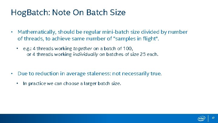
Hog. Batch: Note On Batch Size • Mathematically, should be regular mini-batch size divided by number of threads, to achieve same number of “samples in flight”. • e. g. : 4 threads working together on a batch of 100, or 4 threads working individually on batches of size 25 each. • Due to reduction in average staleness: not necessarily true. • In practice we can choose a larger batch size. 47

Parallel scaling of Strategies Sparse Problem • RCV 1 test dataset: Frequency • Hogwild • • • Better to double frequency than double core count. core-to-core interconnect speedup is needed. Batching • • Dataset Name rcv 1 -test Nearly equivalent to double frequency or core count. This is due to private vectors not causing core-to-core traffic. Examples Features 677, 399 Time (in seconds) to 99. 5% optimal. NNZ 47, 236 Sparsity (%) 49, 556, 258 0. 155 NNZ/Row Range 4 to 1, 224 Avg NNZ/Row 73. 157 48

Raw time data RCV 1 Covtype 49