High Performance networks Contents Some definition Static Network

High Performance networks

Contents • Some definition • Static Network Technologies • Dynamic Network technologies

Overview of networks • Networks to be considered as bidirectional graphs with • nodes : processing elements. • edges: connection between processing elements.

Degree

Diameter

Connectivity

Bisection Width

Blocking

Bandwidth

Static/Dynamic network Technologies

Static network Technologies STATIC NETWORK TECHNOLOGIES • Fixed connection between pairs of nodes • control functions are done by special connection hardware The following network topologies are commonly used: 1 Ring Network 2 Star Connected Network 3 Completely Connected Network 4 Tree Network 5 Mesh Network 6 Hypercube Network.

Dynamic network Technologies • No fixed connection between pairs of nodes. • All nodes are connected via inputs and outputs to a so called switching component. • control functions are connected in the switching component • various routes can be switched The following network topologies are commonly used: 1 Crossbar Network 2 Bus based Network 3 Multistage Interconnection Network.

Linear array • One dimensional network • N nodes and N-1 edges • Degree=2 • Diameter=N-1 • Bisection width=1 • drawback: too slow for large N

Ring • • • two dimensional network N nodes and N edges Degree=2 Diameter=N/2 Bisection width=2 drawback: too slow for large N

Completely connected § § § § two dimensional network N nodes and N(N-1)/2 edges Degree=N-1 Diameter=1 Bisection width=[N/2] Very high fault tolerance drawback: too expensive for large N

Star • • • two dimensional network N nodes and N-1 edges Degree=N-1 Diameter=2 Bisection width=[N/2] drawback: bottleneck in central node

Binary Tree • • • two dimensional network N nodes and N-1 edges Degree=3 Diameter=2 h Bisection width=1 drawback: bottleneck in direction of root(blocking)

Mesh/torus • • K dimensional network N nodes and k(N-r) edges( rxr mesh, r =k Degree=2 k Diameter=k(r-1) Bisection width= High fault tolerance Drawback • Large diameter • Too expensive for k>3

Network Topologies: Linear Arrays Linear arrays: (a) with no wraparound links; (b) with wraparound link. 19

Network Topologies: Two- and Three Dimensional Meshes Two and three dimensional meshes: (a) 2 -D mesh with no wraparound; (b) 2 -D mesh with wraparound link (2 -D torus); and (c) a 3 -D mesh with no wraparound. 20

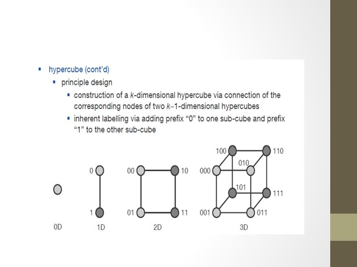
Hypercube

Hypercube routing To go from node x 1 x 2 x 3 to node y 1 y 2 y 3 • Each x and y representing bits • Go to y 1 x 2 x 3 • Then go to y 1 y 2 y 3 if y 1 and x 1 different if y 2 and x 2 different if y 3 and x 3 different Example 101 to 010 101 -> 001 ->011 -> 010

Hypercube Routing 2 • This routing scheme is called e-cube routing algorithm, or leftto-right routing • Example: What is the route taken from node # 13 to node # 42? • 13 (001101)->42(101010)

Hypercube Routing Example • Answer: • 13 (001101)->42(101010) • 13(001101)->45(101101)->41(101001)-> 43(101011)->42(101010)

Dynamic Network topologies

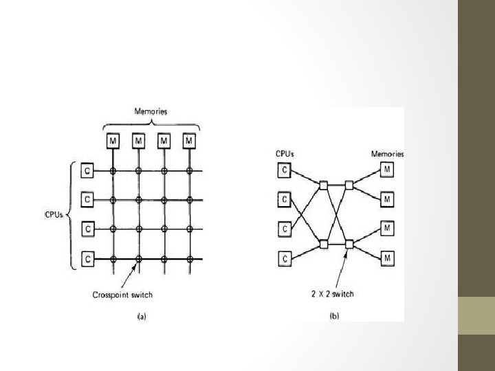
Crossbar

• How many switch points are there in a crossbar switch network that connects p processors to m memory modules?

Network Topologies: Multistage Network • Multistage Networks • Intermediate class of networks between bus-based network and crossbar network • Blocking networks: access to a memory bank by a processor may disallow access to another memory bank by another processor. • More scalable than the bus-based network in terms of performance, more scalable than crossbar network in terms of cost. 31 The schematic of a typical multistage interconnection network.

Network Topologies: Multistage Omega Network • Omega network • Consists of log p stages, p is the number of inputs(processing nodes) and also the number of outputs(memory banks) • Each stage consists of an interconnection pattern that connects p inputs and p outputs: • Perfect shuffle(left rotation): • Each switch has two conncetion modes: • Pass-thought conncetion: the inputs are sent straight through to the outputs • Cross-over connection: the inputs to the switching node are crossed over and then sent out. • Has p/2*log p switching nodes 32

Network Topologies: Multistage Omega Network A complete Omega network with the perfect shuffle interconnects and switches can now be illustrated: A complete omega network connecting eight inputs and eight outputs. An omega network has p/2 × log p switching nodes, and the cost of such a network grows as (p log p). 33