Hierarchical Models Stefan Kiebel Wellcome Dept of Imaging

Hierarchical Models Stefan Kiebel Wellcome Dept. of Imaging Neuroscience University College London

Overview Why hierarchical models? The model Estimation Expectation-Maximization Summary Statistics approach Variance components Examples

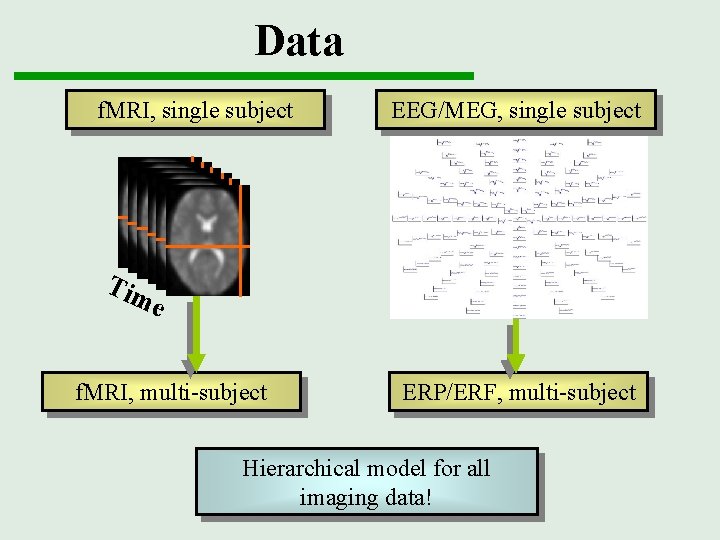
Data f. MRI, single subject EEG/MEG, single subject Tim e f. MRI, multi-subject ERP/ERF, multi-subject Hierarchical model for all imaging data!

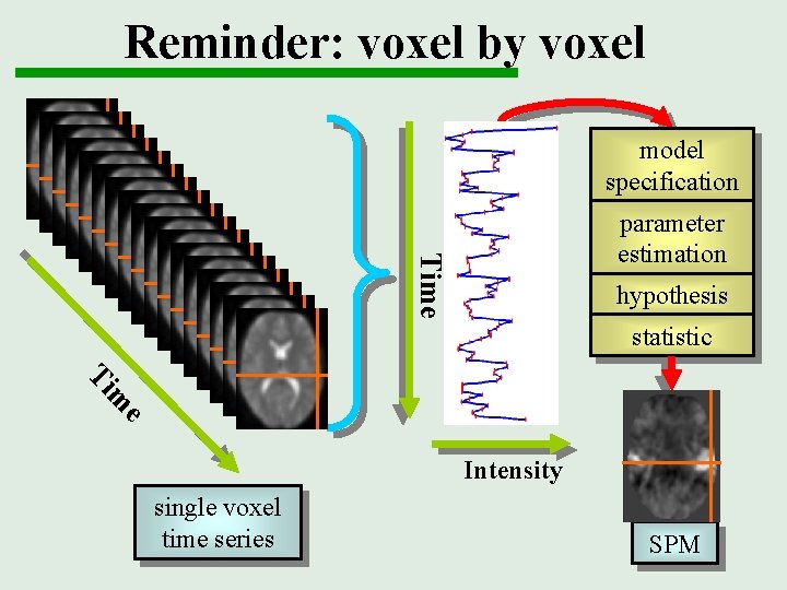
Reminder: voxel by voxel model specification Time parameter estimation hypothesis statistic Ti e m Intensity single voxel time series SPM

Overview Why hierarchical models? The model Estimation Expectation-Maximization Summary Statistics approach Variance components Examples

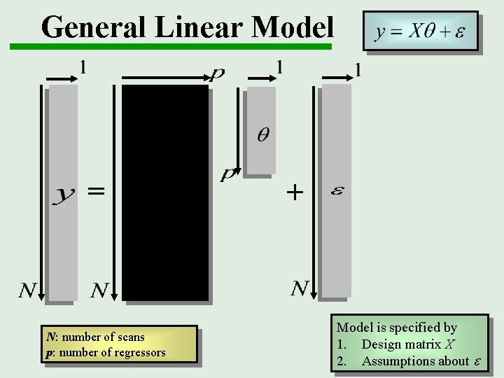
General Linear Model = N: number of scans p: number of regressors + Model is specified by 1. Design matrix X 2. Assumptions about e

Linear hierarchical model Hierarchical model Multiple variance components at each level At each level, distribution of parameters is given by level above. What we don’t know: distribution of parameters and variance parameters.

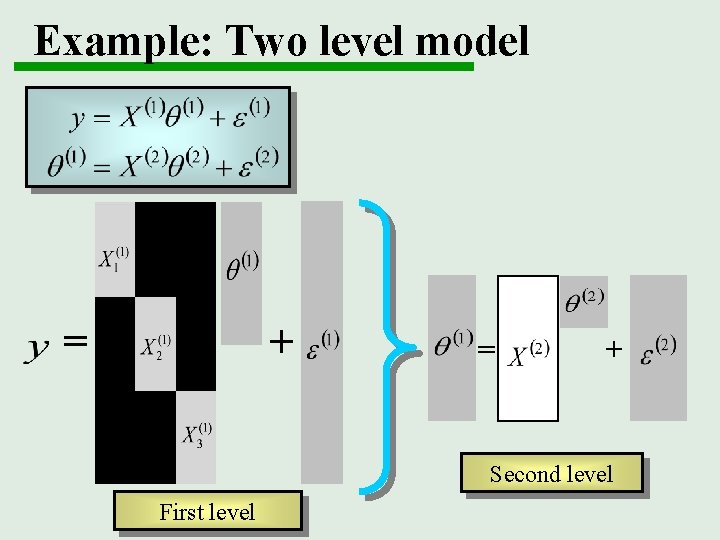
Example: Two level model = + Second level First level

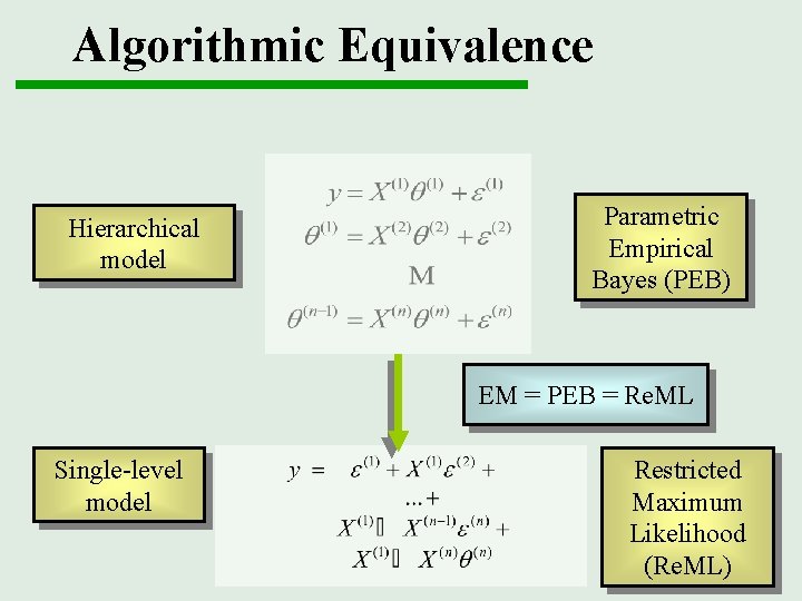
Algorithmic Equivalence Hierarchical model Parametric Empirical Bayes (PEB) EM = PEB = Re. ML Single-level model Restricted Maximum Likelihood (Re. ML)

Overview Why hierarchical models? The model Estimation Expectation-Maximization Summary Statistics approach Variance components Examples

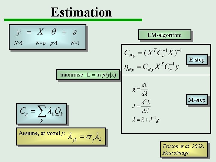
Estimation EM-algorithm E-step M-step Assume, at voxel j: Friston et al. 2002, Neuroimage

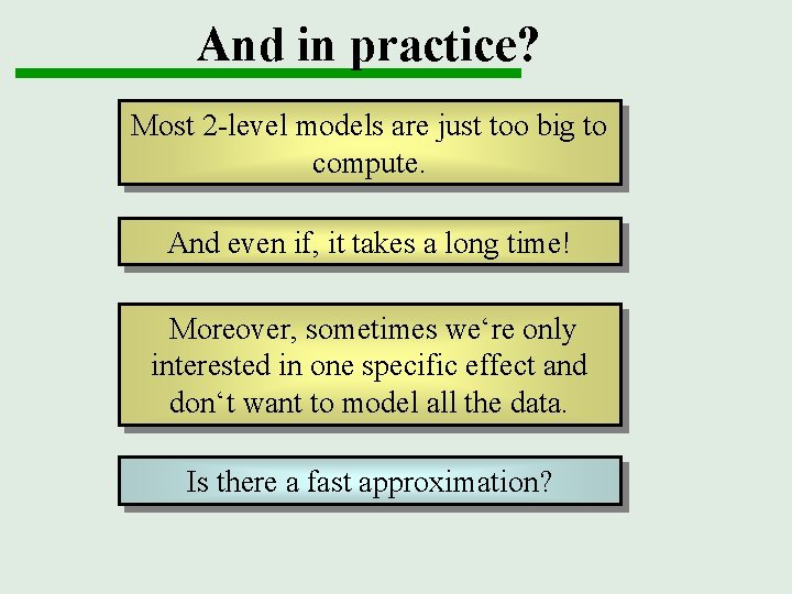
And in practice? Most 2 -level models are just too big to compute. And even if, it takes a long time! Moreover, sometimes we‘re only interested in one specific effect and don‘t want to model all the data. Is there a fast approximation?

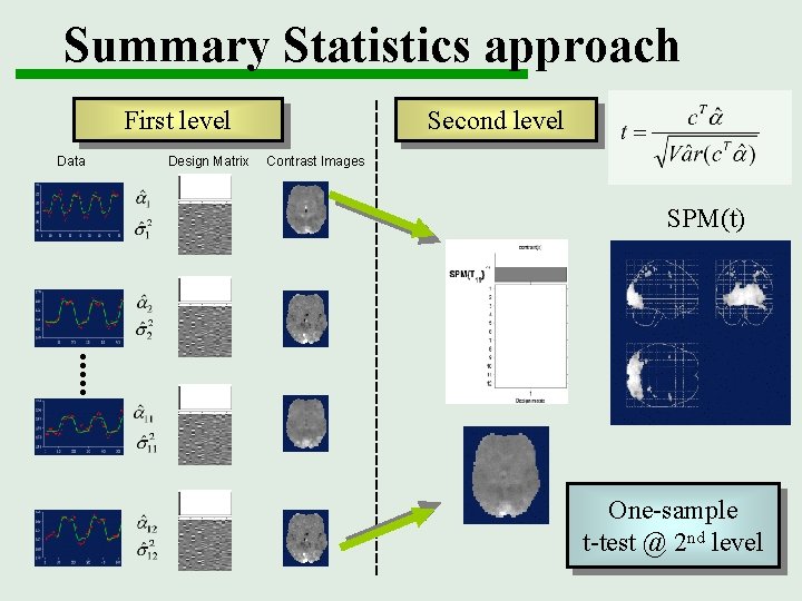
Summary Statistics approach First level Data Design Matrix Second level Contrast Images SPM(t) One-sample t-test @ 2 nd level

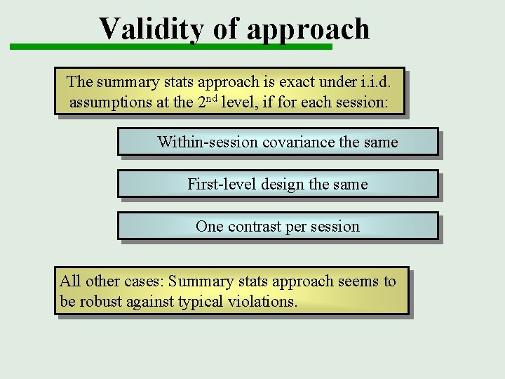
Validity of approach The summary stats approach is exact under i. i. d. assumptions at the 2 nd level, if for each session: Within-session covariance the same First-level design the same One contrast per session All other cases: Summary stats approach seems to be robust against typical violations.

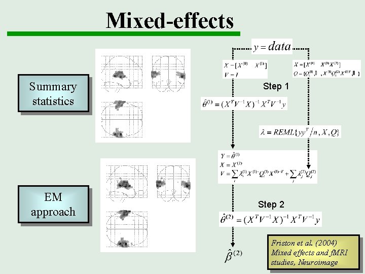
Mixed-effects Summary statistics EM approach Step 1 Step 2 Friston et al. (2004) Mixed effects and f. MRI studies, Neuroimage

Overview Why hierarchical models? The model Estimation Expectation-Maximization Summary Statistics approach Variance components Examples

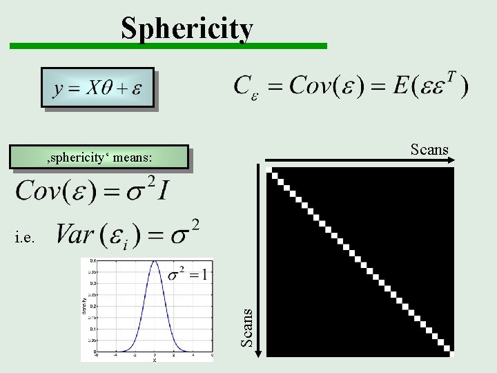
Sphericity Scans ‚sphericity‘ means: Scans i. e.

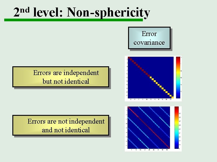
2 nd level: Non-sphericity Error covariance Errors are independent but not identical Errors are not independent and not identical

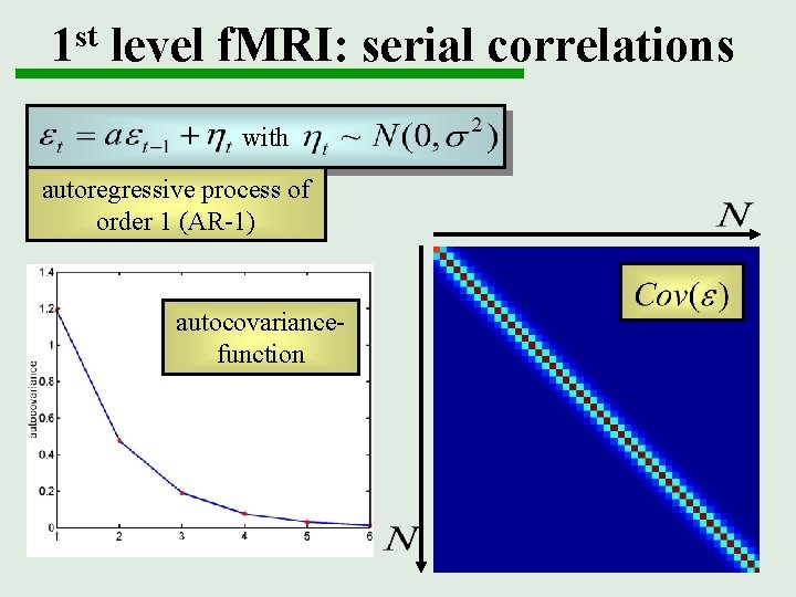
1 st level f. MRI: serial correlations with autoregressive process of order 1 (AR-1) autocovariancefunction

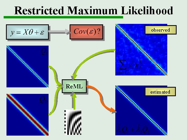
Restricted Maximum Likelihood observed Re. ML estimated

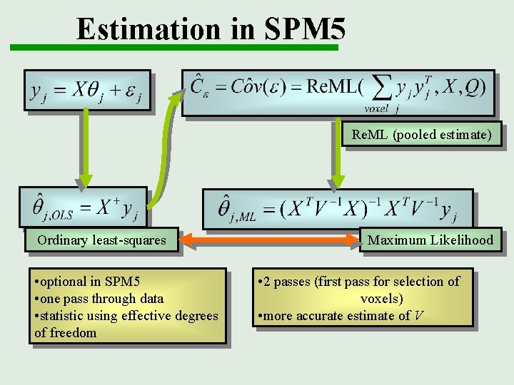
Estimation in SPM 5 Re. ML (pooled estimate) Ordinary least-squares • optional in SPM 5 • one pass through data • statistic using effective degrees of freedom Maximum Likelihood • 2 passes (first pass for selection of voxels) • more accurate estimate of V

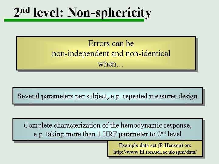
2 nd level: Non-sphericity Errors can be non-independent and non-identical when… Several parameters per subject, e. g. repeated measures design Complete characterization of the hemodynamic response, e. g. taking more than 1 HRF parameter to 2 nd level Example data set (R Henson) on: http: //www. fil. ion. ucl. ac. uk/spm/data/

Overview Why hierarchical models? The model Estimation Expectation-Maximization Summary Statistics approach Variance components Examples

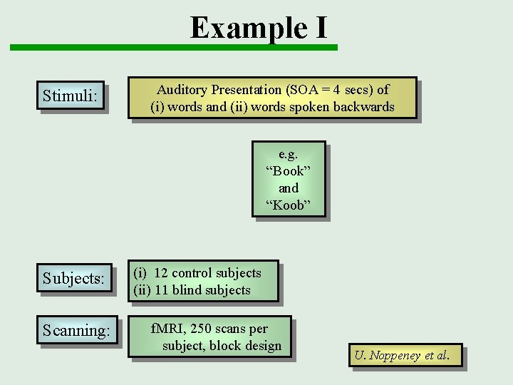
Example I Stimuli: Auditory Presentation (SOA = 4 secs) of (i) words and (ii) words spoken backwards e. g. “Book” and “Koob” Subjects: Scanning: (i) 12 control subjects (ii) 11 blind subjects f. MRI, 250 scans per subject, block design U. Noppeney et al.

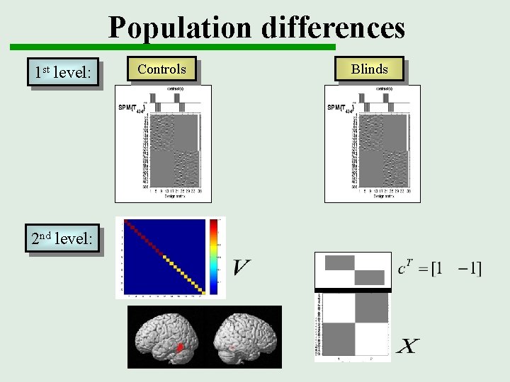
Population differences 1 st level: 2 nd level: Controls Blinds

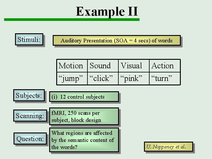
Example II Stimuli: Auditory Presentation (SOA = 4 secs) of words Motion Sound Visual Action “jump” “click” “pink” “turn” Subjects: (i) 12 control subjects Scanning: f. MRI, 250 scans per subject, block design Question: What regions are affected by the semantic content of the words? U. Noppeney et al.

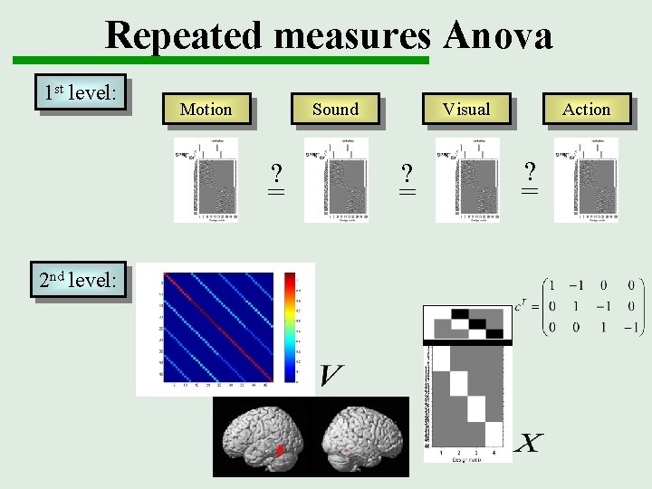
Repeated measures Anova 1 st level: Motion Sound ? = 2 nd level: Visual ? = Action ? =

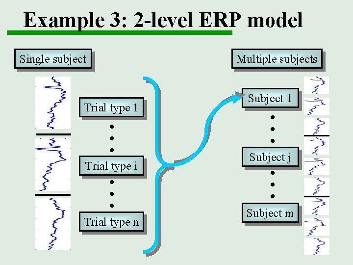
Example 3: 2 -level ERP model Single subject Multiple subjects Trial type 1 Subject j . . . Trial type n . . . Trial type i Subject 1 Subject m

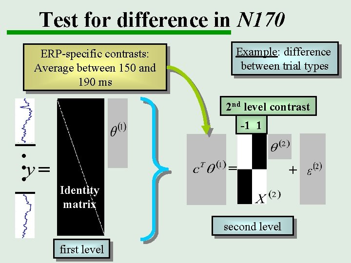
Test for difference in N 170 ERP-specific contrasts: Average between 150 and 190 ms Example: difference between trial types 2 nd level contrast -1 1 . . . = = Identity matrix second level first level +

Some practical points RFX: If not using multi-dimensional contrasts at 2 nd level (Ftests), use a series of 1 -sample t-tests at the 2 nd level. Use mixed-effects model only, if seriously in doubt about validity of summary statistics approach. If using variance components at 2 nd level: Always check your variance components (explore design).

Conclusion Linear hierarchical models are general enough for typical multi-subject imaging data (PET, f. MRI, EEG/MEG). Summary statistics are robust approximation to mixed-effects analysis. To minimize number of variance components to be estimated at 2 nd level, compute relevant contrasts at 1 st level and use simple test at 2 nd level.