HIERARCHICAL CLUSTERING ALGORITHMS v They produce a hierarchy

HIERARCHICAL CLUSTERING ALGORITHMS v They produce a hierarchy of (hard) clusterings instead of a single clustering. v Applications in: Ø Ø Ø Social sciences Biological taxonomy Modern biology Medicine Archaeology Computer science and engineering 1

v Let X={x 1, …, x. N}, xi=[xi 1, …, xil]T. Recall that: Ø In hard clustering each vector belongs exclusively to a single cluster. Ø An m-(hard) clustering of X, , is a partition of X into m sets (clusters) C 1, …, Cm , so that: • • • By the definition: ={Cj, j=1, …m} Ø Definition: A clustering 1 containing k clusters is said to be nested in the clustering 2 containing r (<k) clusters, if each cluster in 1 is a subset of a cluster in 2. We write 1 2 2

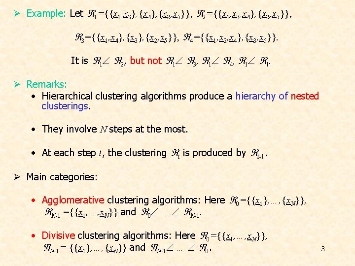
Ø Example: Let 1={{x 1, x 3}, {x 4}, {x 2, x 5}}, 2={{x 1, x 3, x 4}, {x 2, x 5}}, 3={{x 1, x 4}, {x 3}, {x 2, x 5}}, 4={{x 1, x 2, x 4}, {x 3, x 5}}. It is 1 2, but not 1 3, 1 4, 1 1. Ø Remarks: • Hierarchical clustering algorithms produce a hierarchy of nested clusterings. • They involve N steps at the most. • At each step t, the clustering t is produced by t-1. Ø Main categories: • Agglomerative clustering algorithms: Here 0={{x 1}, …, {x. N}}, N-1 ={{x 1, …, x. N}} and 0 … N-1. • Divisive clustering algorithms: Here 0={{x 1, …, x. N}}, N-1= {{x 1}, …, {x. N}} and N-1 … 0. 3

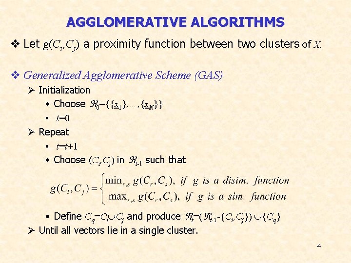
AGGLOMERATIVE ALGORITHMS v Let g(Ci, Cj) a proximity function between two clusters of X. v Generalized Agglomerative Scheme (GAS) Ø Initialization • Choose 0={{x 1}, …, {x. N}} • t=0 Ø Repeat • t=t+1 • Choose (Ci, Cj) in t-1 such that • Define Cq=Ci Cj and produce t=( t-1 -{Ci, Cj}) {Cq} Ø Until all vectors lie in a single cluster. 4

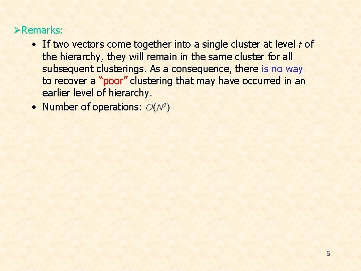
ØRemarks: • If two vectors come together into a single cluster at level t of the hierarchy, they will remain in the same cluster for all subsequent clusterings. As a consequence, there is no way to recover a “poor” clustering that may have occurred in an earlier level of hierarchy. • Number of operations: O(N 3) 5

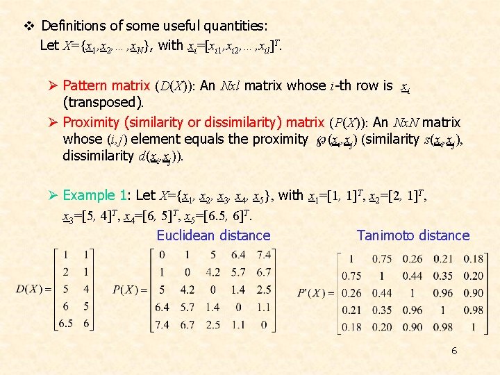
v Definitions of some useful quantities: Let X={x 1, x 2, …, x. N}, with xi=[xi 1, xi 2, …, xil]T. Ø Pattern matrix (D(X)): An Nxl matrix whose i-th row is xi (transposed). Ø Proximity (similarity or dissimilarity) matrix (P(X)): An Nx. N matrix whose (i, j) element equals the proximity (xi, xj) (similarity s(xi, xj), dissimilarity d(xi, xj)). Ø Example 1: Let X={x 1, x 2, x 3, x 4, x 5}, with x 1=[1, 1]T, x 2=[2, 1]T, x 3=[5, 4]T, x 4=[6, 5]T, x 5=[6. 5, 6]T. Euclidean distance Tanimoto distance 6

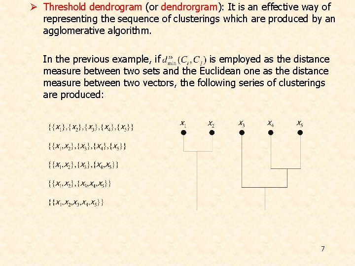
Ø Threshold dendrogram (or dendrorgram): It is an effective way of representing the sequence of clusterings which are produced by an agglomerative algorithm. In the previous example, if is employed as the distance measure between two sets and the Euclidean one as the distance measure between two vectors, the following series of clusterings are produced: 7

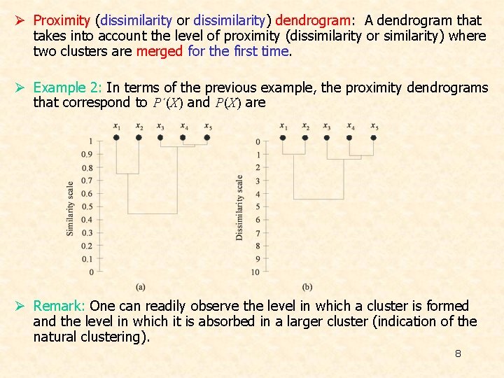
Ø Proximity (dissimilarity or dissimilarity) dendrogram: A dendrogram that takes into account the level of proximity (dissimilarity or similarity) where two clusters are merged for the first time. Ø Example 2: In terms of the previous example, the proximity dendrograms that correspond to P΄(X) and P(X) are Ø Remark: One can readily observe the level in which a cluster is formed and the level in which it is absorbed in a larger cluster (indication of the natural clustering). 8

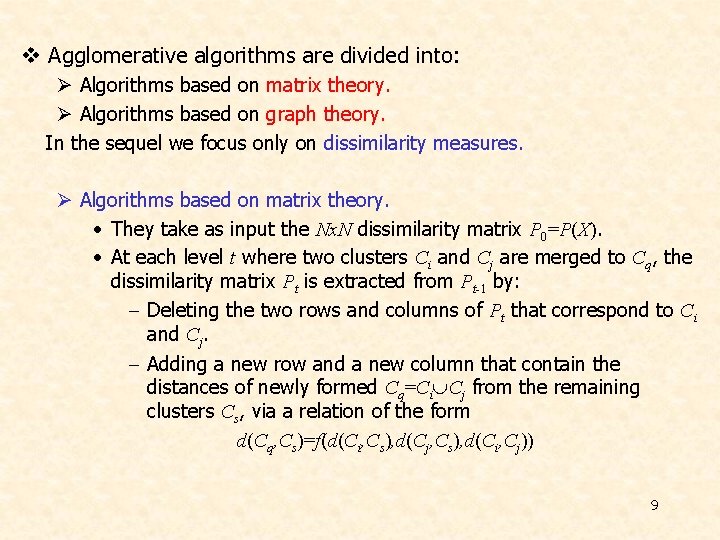
v Agglomerative algorithms are divided into: Ø Algorithms based on matrix theory. Ø Algorithms based on graph theory. In the sequel we focus only on dissimilarity measures. Ø Algorithms based on matrix theory. • They take as input the Nx. N dissimilarity matrix P 0=P(X). • At each level t where two clusters Ci and Cj are merged to Cq, the dissimilarity matrix Pt is extracted from Pt-1 by: - Deleting the two rows and columns of Pt that correspond to Ci and Cj. - Adding a new row and a new column that contain the distances of newly formed Cq=Ci Cj from the remaining clusters Cs, via a relation of the form d(Cq, Cs)=f(d(Ci, Cs), d(Cj, Cs), d(Ci, Cj)) 9

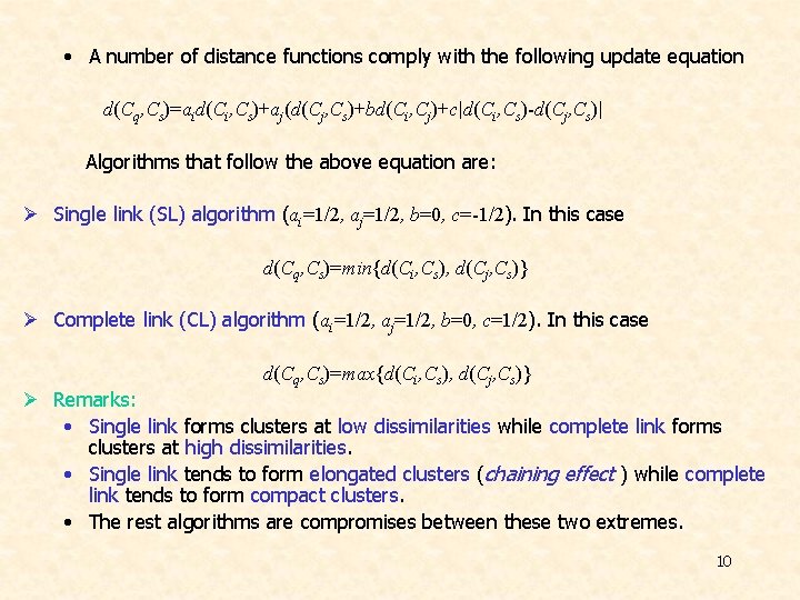
• A number of distance functions comply with the following update equation d(Cq, Cs)=aid(Ci, Cs)+aj(d(Cj, Cs)+bd(Ci, Cj)+c|d(Ci, Cs)-d(Cj, Cs)| Algorithms that follow the above equation are: Ø Single link (SL) algorithm (ai=1/2, aj=1/2, b=0, c=-1/2). In this case d(Cq, Cs)=min{d(Ci, Cs), d(Cj, Cs)} Ø Complete link (CL) algorithm (ai=1/2, aj=1/2, b=0, c=1/2). In this case d(Cq, Cs)=max{d(Ci, Cs), d(Cj, Cs)} Ø Remarks: • Single link forms clusters at low dissimilarities while complete link forms clusters at high dissimilarities. • Single link tends to form elongated clusters (chaining effect ) while complete link tends to form compact clusters. • The rest algorithms are compromises between these two extremes. 10

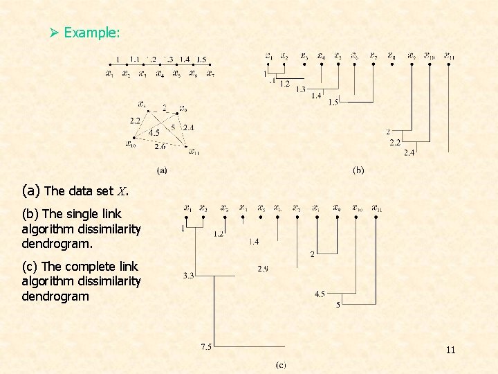
Ø Example: (a) The data set X. (b) The single link algorithm dissimilarity dendrogram. (c) The complete link algorithm dissimilarity dendrogram 11

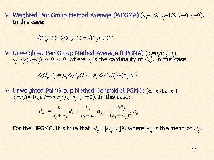
Ø Weighted Pair Group Method Average (WPGMA) (ai=1/2, aj=1/2, b=0, c=0). In this case: d(Cq, Cs)=(d(Ci, Cs) + d(Cj, Cs))/2 Ø Unweighted Pair Group Method Average (UPGMA) (ai=ni/(ni+nj), aj=nj/(ni+nj), b=0, c=0, where ni is the cardinality of Ci). In this case: d(Cq, Cs)=(ni d(Ci, Cs) + nj d(Cj, Cs))/(ni+nj) Ø Unweighted Pair Group Method Centroid (UPGMC) (ai=ni/(ni+nj), aj=nj/(ni+nj), b=-ni nj/(ni+nj)2, c=0). In this case: For the UPGMC, it is true that dqs=||mq-ms||2, where mq is the mean of Cq. 12

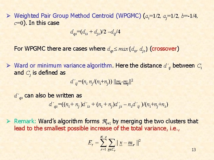
Ø Weighted Pair Group Method Centroid (WPGMC) (ai=1/2, aj=1/2, b=-1/4, c=0). In this case dqs=(dis + djs)/2 –dij/4 For WPGMC there are cases where dqs max{dis, djs} (crossover) Ø Ward or minimum variance algorithm. Here the distance d´ij between Ci and Cj is defined as d´ij=(ni nj/(ni+nj)) ||mi-mj||2 d´qs can also be written as d´qs=((ni + nj )d´is + (ni + nj)d´js – nsd´ij )/(ni+nj+ns) Ø Remark: Ward’s algorithm forms t+1 by merging the two clusters that lead to the smallest possible increase of the total variance, i. e. , 13

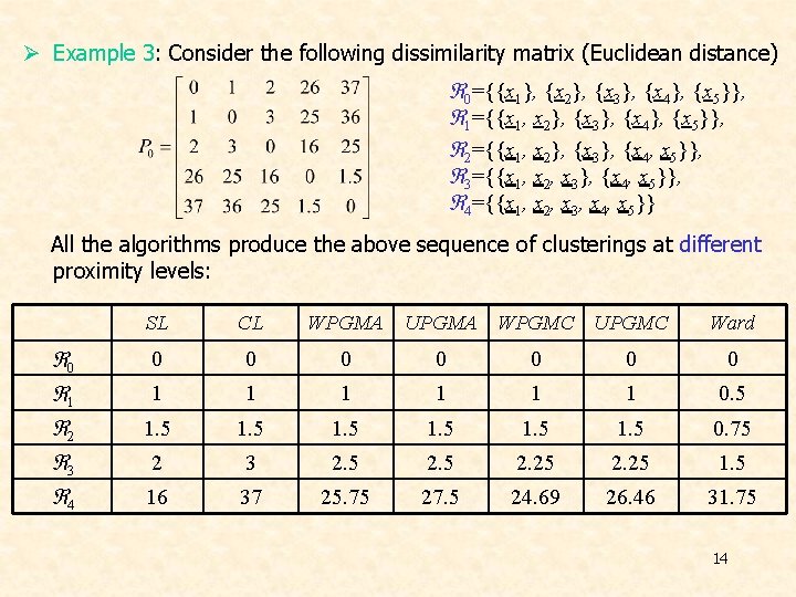
Ø Example 3: Consider the following dissimilarity matrix (Euclidean distance) 0={{x 1}, {x 2}, {x 3}, {x 4}, {x 5}}, 1={{x 1, x 2}, {x 3}, {x 4}, {x 5}}, 2={{x 1, x 2}, {x 3}, {x 4, x 5}}, 3={{x 1, x 2, x 3}, {x 4, x 5}}, 4={{x 1, x 2, x 3, x 4, x 5}} All the algorithms produce the above sequence of clusterings at different proximity levels: 0 1 2 3 4 SL CL WPGMA UPGMA WPGMC UPGMC Ward 0 0 0 0 1 1 1 0. 5 1. 5 0. 75 2 3 2. 5 2. 25 1. 5 16 37 25. 75 27. 5 24. 69 26. 46 31. 75 14

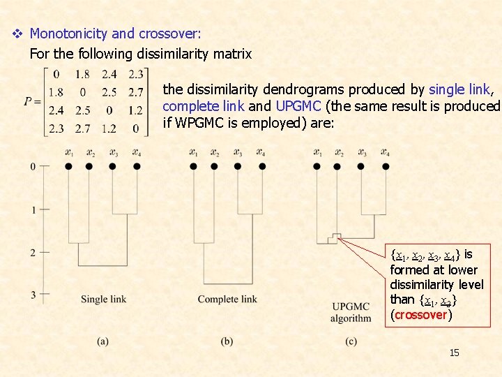
v Monotonicity and crossover: For the following dissimilarity matrix the dissimilarity dendrograms produced by single link, complete link and UPGMC (the same result is produced if WPGMC is employed) are: {x 1, x 2, x 3, x 4} is formed at lower dissimilarity level than {x 1, x 2} (crossover) 15

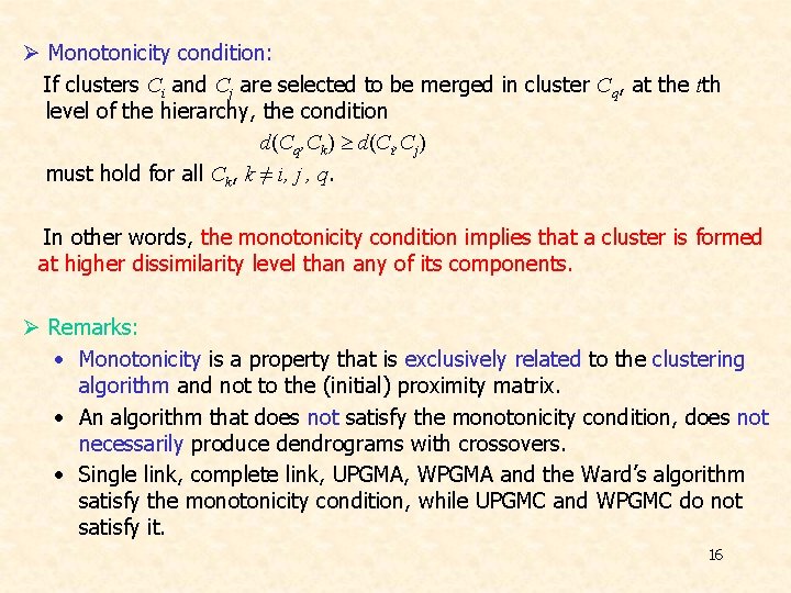
Ø Monotonicity condition: If clusters Ci and Cj are selected to be merged in cluster Cq, at the tth level of the hierarchy, the condition d(Cq, Ck) d(Ci, Cj) must hold for all Ck, k ≠ i, j , q. In other words, the monotonicity condition implies that a cluster is formed at higher dissimilarity level than any of its components. Ø Remarks: • Monotonicity is a property that is exclusively related to the clustering algorithm and not to the (initial) proximity matrix. • An algorithm that does not satisfy the monotonicity condition, does not necessarily produce dendrograms with crossovers. • Single link, complete link, UPGMA, WPGMA and the Ward’s algorithm satisfy the monotonicity condition, while UPGMC and WPGMC do not satisfy it. 16

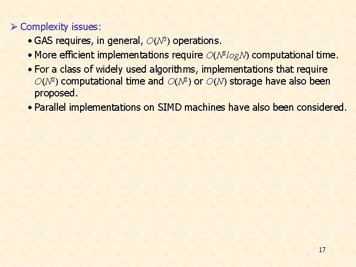
Ø Complexity issues: • GAS requires, in general, O(N 3) operations. • More efficient implementations require O(N 2 log. N) computational time. • For a class of widely used algorithms, implementations that require O(N 2) computational time and O(N 2) or O(N) storage have also been proposed. • Parallel implementations on SIMD machines have also been considered. 17

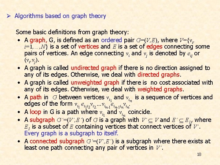
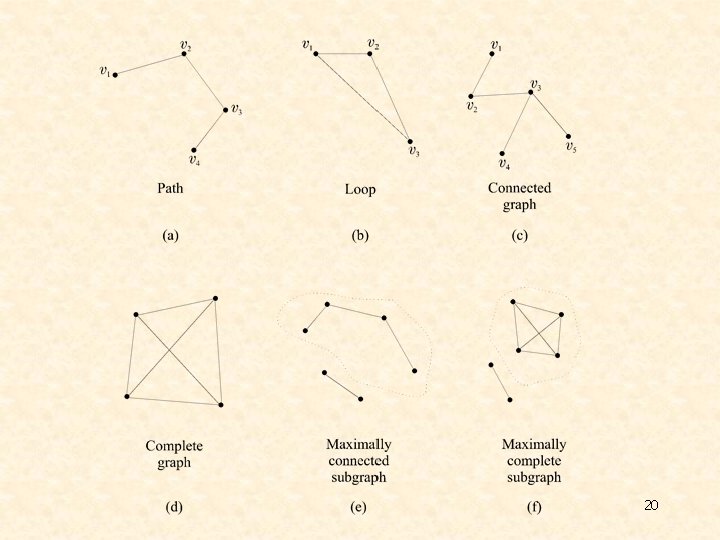
Ø Algorithms based on graph theory Some basic definitions from graph theory: • A graph, G, is defined as an ordered pair G=(V, E), where V={vi, i=1, …, N} is a set of vertices and E is a set of edges connecting some pairs of vertices. An edge connecting vi and vj is denoted by eij or (vi, vj). • A graph is called undirected graph if there is no direction assigned to any of its edges. Otherwise, we deal with directed graphs. • A graph is called unweighted graph if there is no cost associated with any of its edges. Otherwise, we deal with weighted graphs. • A path in G between vertices vi 1 and vin is a sequence of vertices and edges of the form vi 1 ei 1 i 2 vi 2. . vin-1 ein-1 invin. • A loop in G is a path where vi 1 and vin coincide. • A subgraph G´=(V´, E´) of G is a graph with V´ V and E´ E 1, where E 1 is a subset of E containing vertices that connect vertices of V´. Every graph is a subgraph to itself. • A connected subgraph G´=(V´, E´) is a subgraph where there exists at least one path connecting any pair of vertices in V´. 18

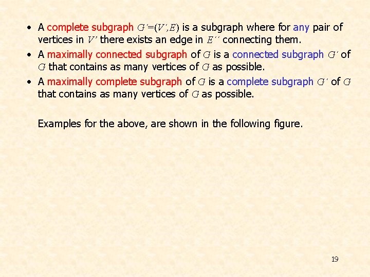
• A complete subgraph G´=(V´, E) is a subgraph where for any pair of vertices in V’ there exists an edge in E´´ connecting them. • A maximally connected subgraph of G is a connected subgraph G´ of G that contains as many vertices of G as possible. • A maximally complete subgraph of G is a complete subgraph G´ of G that contains as many vertices of G as possible. Examples for the above, are shown in the following figure. 19

20

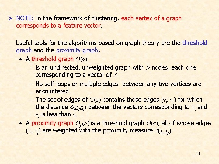
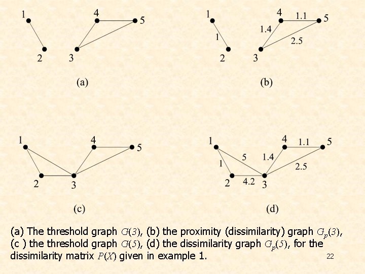
Ø NOTE: In the framework of clustering, each vertex of a graph corresponds to a feature vector. Useful tools for the algorithms based on graph theory are threshold graph and the proximity graph. • A threshold graph G(a) - is an undirected, unweighted graph with N nodes, each one corresponding to a vector of X. - No self-loops or multiple edges between any two vertices are encountered. - The set of edges of G(a) contains those edges (vi, vj) for which the distance d(xi, xj) between the vectors corresponding to vi and vj is less than a. • A proximity graph Gp(a) is a threshold graph G(a), all of whose edges (vi, vj) are weighted with the proximity measure d(xi, xj). 21

(a) The threshold graph G(3), (b) the proximity (dissimilarity) graph Gp(3), (c ) the threshold graph G(5), (d) the dissimilarity graph Gp(5), for the 22 dissimilarity matrix P(X) given in example 1.

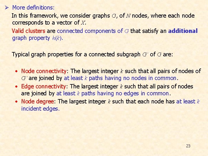
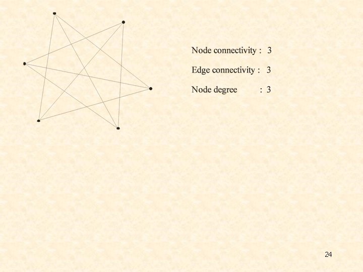
Ø More definitions: In this framework, we consider graphs G, of N nodes, where each node corresponds to a vector of X. Valid clusters are connected components of G that satisfy an additional graph property h(k). Typical graph properties for a connected subgraph G´ of G are: • Node connectivity: The largest integer k such that all pairs of nodes of G´ are joined by at least k paths having no nodes in common. • Edge connectivity: The largest integer k such that all pairs of nodes are joined by at least k paths having no edges in common. • Node degree: The largest integer k such that each node has at least k incident edges. 23

24

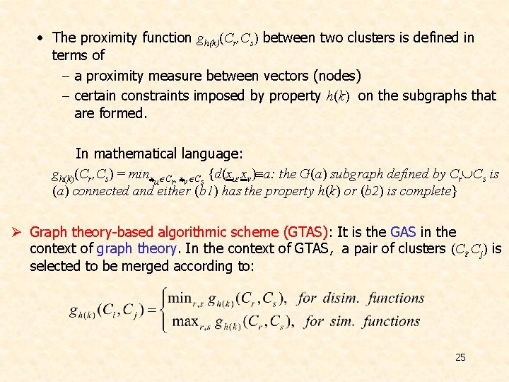
• The proximity function gh(k)(Cr, Cs) between two clusters is defined in terms of - a proximity measure between vectors (nodes) - certain constraints imposed by property h(k) on the subgraphs that are formed. In mathematical language: gh(k)(Cr, Cs) = minxu Cr, xv Cs {d(xu, xv) a: the G(a) subgraph defined by Cr Cs is (a) connected and either (b 1) has the property h(k) or (b 2) is complete} Ø Graph theory-based algorithmic scheme (GTAS): It is the GAS in the context of graph theory. In the context of GTAS, a pair of clusters (Ci, Cj) is selected to be merged according to: 25

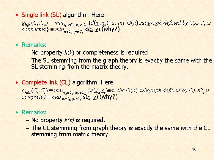
• Single link (SL) algorithm. Here gh(k)(Cr, Cs) = minxu Cr, xv Cs {d(xu, xv) a: the G(a) subgraph defined by Cr Cs is connected} minx Cr, y Cs d(x, y) (why? ) • Remarks: - No property h(k) or completeness is required. - The SL stemming from the graph theory is exactly the same with the SL stemming from the matrix theory. • Complete link (CL) algorithm. Here gh(k)(Cr, Cs) = minxu Cr, xv Cs {d(xu, xv) a: the G(a) subgraph defined by Cr Cs is complete} maxx Cr, y Cs d(x, y) (why? ) • Remarks: - No property h(k) is required. - The CL stemming from graph theory is exactly the same with the CL stemming from matrix theory. 26

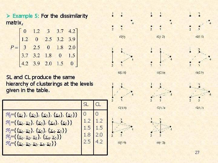
Ø Example 5: For the dissimilarity matrix, SL and CL produce the same hierarchy of clusterings at the levels given in the table. 0={{x 1}, {x 2}, {x 3}, {x 4}, {x 5}} 1={{x 1, x 2}, {x 3}, {x 4}, {x 5}} 2={{x 1, x 2}, {x 3}, {x 4, x 5}} 3={{x 1, x 2, x 3}, {x 4, x 5}} 4={{x 1, x 2, x 3, x 4, x 5}} SL CL 0 1. 2 1. 5 1. 8 2. 5 0 1. 2 1. 5 2. 0 4. 2 27

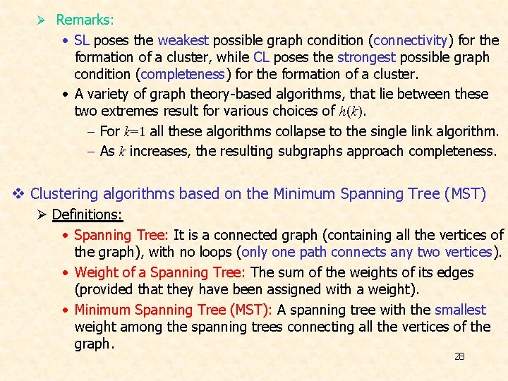
Ø Remarks: • SL poses the weakest possible graph condition (connectivity) for the formation of a cluster, while CL poses the strongest possible graph condition (completeness) for the formation of a cluster. • A variety of graph theory-based algorithms, that lie between these two extremes result for various choices of h(k). - For k=1 all these algorithms collapse to the single link algorithm. - As k increases, the resulting subgraphs approach completeness. v Clustering algorithms based on the Minimum Spanning Tree (MST) Ø Definitions: • Spanning Tree: It is a connected graph (containing all the vertices of the graph), with no loops (only one path connects any two vertices). • Weight of a Spanning Tree: The sum of the weights of its edges (provided that they have been assigned with a weight). • Minimum Spanning Tree (MST): A spanning tree with the smallest weight among the spanning trees connecting all the vertices of the graph. 28

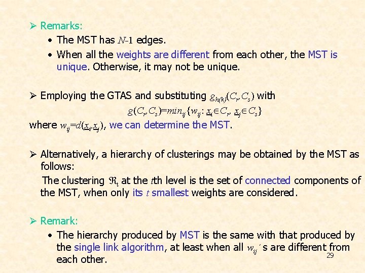
Ø Remarks: • The MST has N-1 edges. • When all the weights are different from each other, the MST is unique. Otherwise, it may not be unique. Ø Employing the GTAS and substituting gh(k)(Cr, Cs) with g(Cr, Cs)=minij{wij: xi Cr, xj Cs} where wij=d(xi, xj), we can determine the MST. Ø Alternatively, a hierarchy of clusterings may be obtained by the MST as follows: The clustering t at the tth level is the set of connected components of the MST, when only its t smallest weights are considered. Ø Remark: • The hierarchy produced by MST is the same with that produced by the single link algorithm, at least when all wij´ s are different from 29 each other.

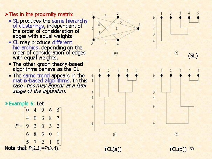
ØTies in the proximity matrix • SL produces the same hierarchy of clusterings, independent of the order of consideration of edges with equal weights. • CL may produce different hierarchies, depending on the order of consideration of edges with equal weights. • The other graph theory-based algorithms behave as the CL. • The same trend appears in the matrix-based algorithms. In this case, ties may appear at a later stage of the algorithm. (SL) ØExample 6: Let Note that P(2, 3)=P(3, 4). (CL(a)) (CL(b)) 30

DIVISIVE ALGORITHMS Ø Let g(Ci, Cj) be a dissimilarity function between two clusters. Ø Let Ctj denote the jth cluster of the tth clustering t, t=0, …, N-1, j=1, …, t+1. 31

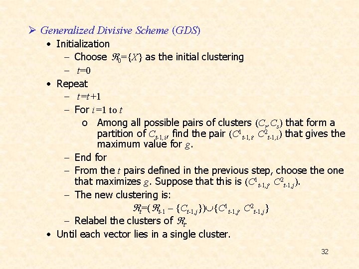
Ø Generalized Divisive Scheme (GDS) • Initialization - Choose 0={X} as the initial clustering - t=0 • Repeat - t=t+1 - For i=1 to t o Among all possible pairs of clusters (Cr, Cs) that form a partition of Ct-1, i, find the pair (C 1 t-1, i, C 2 t-1, i) that gives the maximum value for g. - End for - From the t pairs defined in the previous step, choose the one that maximizes g. Suppose that this is (C 1 t-1, j, C 2 t-1, j). - The new clustering is: t=( t-1 – {Ct-1, j}) {C 1 t-1, j, C 2 t-1, j} - Relabel the clusters of t. • Until each vector lies in a single cluster. 32

Ø Remarks: • Different choices of g give rise to different algorithms. • The GDS is computationally very demanding even for small N. • Algorithms that rule out many partitions as not “reasonable”, under a prespecified criterion, have also been proposed. • Algorithms where the splitting of the clusters is based on all features of the feature vectors are called polythetic algorithms. Otherwise, if the splitting is based on a single feature at each step, the algorithms are called monothetic algorithms. 33

HIERARCHICAL ALGORITHMS FOR LARGE DATA SETS v Since the number of operations required by GAS is greater than O(N 2), algorithms resulting by GAS are prohibitive for very large data sets encountered, for example, in web mining and bioinformatics. To overcome this drawback, various hierarchical algorithms of special type have been developed that are tailored to handle large data sets. Typical examples are: Ø The CURE algorithm. Ø The ROCK algorithm. Ø The Chameleon algorithm. 34

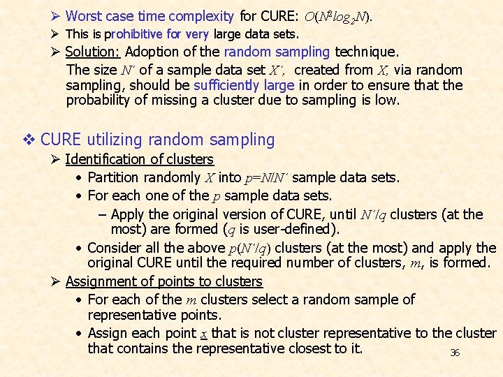
v The CURE (Clustering Using Representatives) algorithm In CURE: Ø Each cluster C is represented by a set of k > 1 representatives, denoted by RC. Ø These representatives try to “capture” the shape of the cluster. Ø They are chosen at the “border” of the cluster and then, they are pushed toward its mean, in order to discard the irregularities of the border. More specifically, RC is determined as follows: Ø Select x C, with the maximum distance from the mean m. C of C and set RC={x} Ø For i=2 to min{k, n. C} (n. C is the number of points in C) • Determine y C-RC that lies farthest from the points of RC and set RC= RC {y}. Ø Shrink the points x RC toward the mean m. C in C by a factor a. That is x=(1 -a) x+a m. C , x RC. CURE is a special case of GAS where the distance between two clusters is defined as: 35

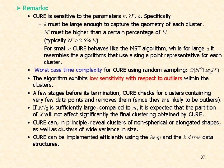
Ø Worst case time complexity for CURE: O(N 2 log 2 N). Ø This is prohibitive for very large data sets. Ø Solution: Adoption of the random sampling technique. The size N´ of a sample data set X´, created from X, via random sampling, should be sufficiently large in order to ensure that the probability of missing a cluster due to sampling is low. v CURE utilizing random sampling Ø Identification of clusters • Partition randomly X into p=N/N´ sample data sets. • For each one of the p sample data sets. – Apply the original version of CURE, until N´/q clusters (at the most) are formed (q is user-defined). • Consider all the above p(N´/q) clusters (at the most) and apply the original CURE until the required number of clusters, m, is formed. Ø Assignment of points to clusters • For each of the m clusters select a random sample of representative points. • Assign each point x that is not cluster representative to the cluster that contains the representative closest to it. 36

Ø Remarks: • CURE is sensitive to the parameters k, N´, a. Specifically: - k must be large enough to capture the geometry of each cluster. - N´ must be higher than a certain percentage of N (typically N´ 2. 5% N) - For small a CURE behaves like the MST algorithm, while for large a it resembles the algorithms that use a single point representative for each cluster. • Worst case time complexity for CURE using random sampling: O(N´ 2 log 2 N´) • The algorithm exhibits low sensitivity with respect to outliers within the clusters. • A few stages before its termination, CURE checks for clusters containing very few data points and removes them (since they are likely to be outliers). • If N´/q is sufficiently large, compared to m, it is expected that the partition of X will not affect significantly the final clustering obtained by CURE. • CURE can, in principle, reveal clusters of non-spherical or elongated shapes, as well as clusters of wide variance in size. • CURE can be implemented efficiently using the heap and the k-d tree data structures. 37

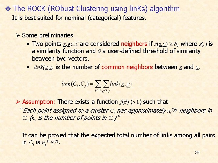
v The ROCK (RObust Clustering using lin. Ks) algorithm It is best suited for nominal (categorical) features. Ø Some preliminaries • Two points x, y X are considered neighbors if s(x, y) θ, where s(. ) is a similarity function and θ a user-defined threshold of similarity between two vectors. • link(x, y) is the number of common neighbors between x and y. Ø Assumption: There exists a function f(θ) (<1) such that: “Each point assigned to a cluster Ci has approximately nif(θ) neighbors in Ci (ni is the number of points in Ci) ” It can be proved that the expected total number of links among all pairs in Ci is ni 1+2 f(θ). 38

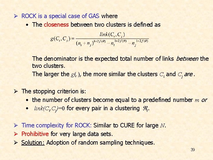
Ø ROCK is a special case of GAS where • The closeness between two clusters is defined as The denominator is the expected total number of links between the two clusters. The larger the g(. ), the more similar the clusters Ci and Cj are. Ø The stopping criterion is: • the number of clusters become equal to a predefined number m or • link(Ci, Cj)=0 for every pair in a clustering t. Ø Time complexity for ROCK: Similar to CURE for large N. Ø Prohibitive for very large data sets. Ø Solution: Adoption of random sampling techniques. 39

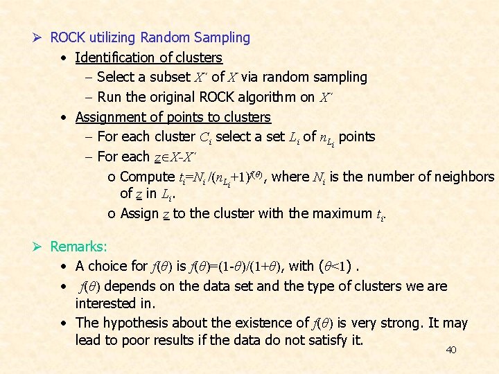
Ø ROCK utilizing Random Sampling • Identification of clusters - Select a subset X´ of X via random sampling - Run the original ROCK algorithm on X´ • Assignment of points to clusters - For each cluster Ci select a set Li of n. Li points - For each z X-X´ o Compute ti=Ni /(n. Li+1)f(θ), where Ni is the number of neighbors of z in Li. o Assign z to the cluster with the maximum ti. Ø Remarks: • A choice for f(θ) is f(θ)=(1 -θ)/(1+θ), with (θ<1). • f(θ) depends on the data set and the type of clusters we are interested in. • The hypothesis about the existence of f(θ) is very strong. It may lead to poor results if the data do not satisfy it. 40

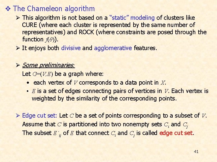
v The Chameleon algorithm Ø This algorithm is not based on a “static” modeling of clusters like CURE (where each cluster is represented by the same number of representatives) and ROCK (where constraints are posed through the function f(θ)). Ø It enjoys both divisive and agglomerative features. Ø Some preliminaries: Let G=(V, E) be a graph where: • each vertex of V corresponds to a data point in X. • E is a set of edges connecting pairs of vertices in V. Each vertex is weighted by the similarity of the corresponding points. Ø Edge cut set: Let C be a set of points corresponding to a subset of V. Assume that C is partitioned into two nonempty sets Ci and Cj The subset E´ij of E that connect Ci and Cj is called edge cut set. 41

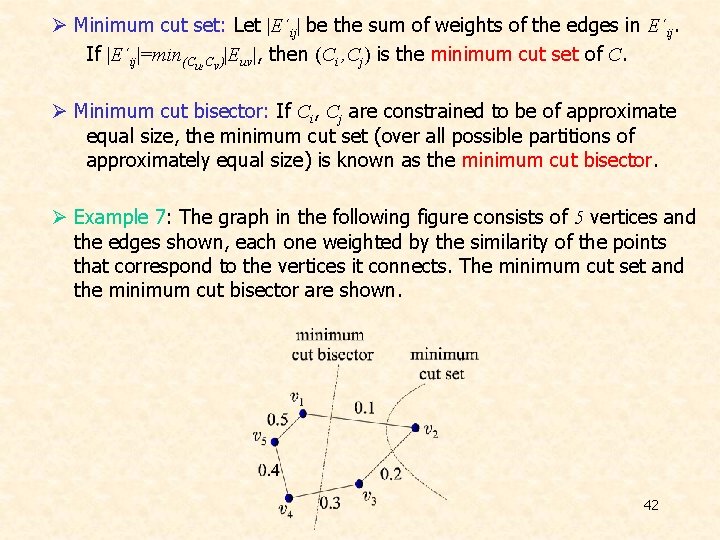
Ø Minimum cut set: Let |E´ij| be the sum of weights of the edges in E´ij. If |E´ij|=min(Cu, Cv)|Euv|, then (Ci , Cj) is the minimum cut set of C. Ø Minimum cut bisector: If Ci, Cj are constrained to be of approximate equal size, the minimum cut set (over all possible partitions of approximately equal size) is known as the minimum cut bisector. Ø Example 7: The graph in the following figure consists of 5 vertices and the edges shown, each one weighted by the similarity of the points that correspond to the vertices it connects. The minimum cut set and the minimum cut bisector are shown. 42

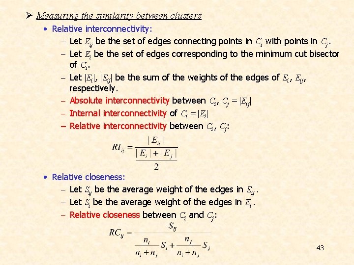
Ø Measuring the similarity between clusters • Relative interconnectivity: - Let Eij be the set of edges connecting points in Ci with points in Cj. - Let Ei be the set of edges corresponding to the minimum cut bisector of Ci. - Let |Ei|, |Eij| be the sum of the weights of the edges of Ei, Eij, respectively. - Absolute interconnectivity between Ci, Cj = |Eij| - Internal interconnectivity of Ci = |Ei| – Relative interconnectivity between Ci, Cj: • Relative closeness: - Let Sij be the average weight of the edges in Eij. - Let Si be the average weight of the edges in Ei. - Relative closeness between Ci and Cj: 43

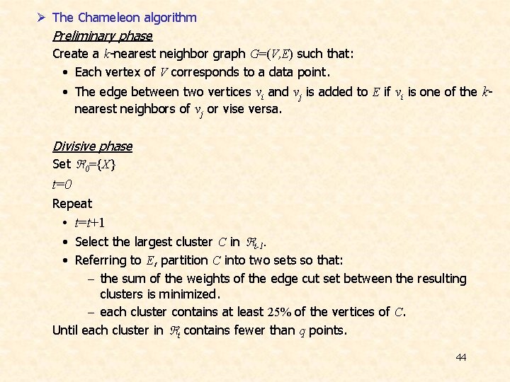
Ø The Chameleon algorithm Preliminary phase Create a k-nearest neighbor graph G=(V, E) such that: • Each vertex of V corresponds to a data point. • The edge between two vertices vi and vj is added to E if vi is one of the knearest neighbors of vj or vise versa. Divisive phase Set 0={X} t=0 Repeat • t=t+1 • Select the largest cluster C in t-1. • Referring to E, partition C into two sets so that: - the sum of the weights of the edge cut set between the resulting clusters is minimized. - each cluster contains at least 25% of the vertices of C. Until each cluster in t contains fewer than q points. 44

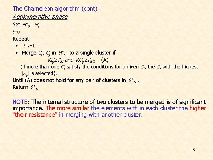
The Chameleon algorithm (cont) Agglomerative phase Set ΄0= t t=0 Repeat • t=t+1 • Merge Ci, Cj in ’t-1 to a single cluster if RIij TRI and RCij TRC (A) (if more than one Cj satisfy the conditions for a given Ci, the Cj with the highest |Eij| is selected). Until (A) does not hold for any pair of clusters in ΄t-1. Return ΄t-1 ΝΟΤΕ: The internal structure of two clusters to be merged is of significant importance. The more similar the elements with in each cluster the higher “their resistance” in merging with another cluster. 45

Ø Remarks: • Condition (A) can be replaced by max(Ci, Cj) RIij RCija • Chameleon is not very sensitive to the choice of the user-defined parameters k (typically it is selected between 5 and 20), q (typically chosen in the range 1 to 5% of the total number of data points), TRI, TRC and/or a. • Chameleon is well suited for large data sets (better estimation of |Eij|, |Ei|, Sij, Si) • For large N, the worst-case time complexity of the algorithm is O(N(log 2 N+m)), where m is the number of clusters formed by the divisive phase. 46

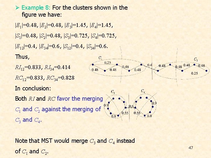
Ø Example 8: For the clusters shown in the figure we have: |E 1|=0. 48, |E 2|=0. 48, |E 3|=1. 45, |E 4|=1. 45, |S 1|=0. 48, |S 2|=0. 48, |S 3|=0. 725, |S 4|=0. 725, |E 12|=0. 4, |E 34|=0. 6, |S 12|=0. 4, |S 34|=0. 6. Thus, RI 12=0. 833, RI 34=0. 414 RC 12=0. 833, RC 34=0. 828 In conclusion: Both RI and RC favor the merging C 1 and C 2 against the merging of C 3 and C 4. Note that MST would merge C 3 and C 4 instead of C 1 and C 2. 47

CHOICE OF THE BEST NUMBER OF CLUSTERS v A major issue associated with hierarchical algorithms is: “How the clustering that best fits the data is extracted from a hierarchy of clusterings? ” Some approaches: Ø Search in the proximity dendrogram for clusters that have a large lifetime (the difference between the proximity level at which a cluster is created and the proximity level at which it is absorbed into a larger cluster (however, this method involves human subjectivity)). Ø Define a function h(C) that measures the dissimilarity between the vectors of the same cluster C. Let be an appropriate threshold for h(C). Then t is the final clustering if there exists a cluster C in t+1 with dissimilarity between its vectors (h(C)) greater than (extrinsic method). The final clustering t must satisfy the following condition: dssmin(Ci, Cj)> max{h(Ci), h(Cj)}, Ci, Cj t In words, in the final clustering, the dissimilarity between every pair of clusters is larger than the “self-similarity” of each one of them (intrinsic 48 method).