Hidden Markov Models Probabilistic Reasoning Over Time Natural

Hidden Markov Models: Probabilistic Reasoning Over Time Natural Language Processing CMSC 25000 February 22, 2005

Agenda • Hidden Markov Models – Uncertain observation – Temporal Context – Recognition: Viterbi – Training the model: Baum-Welch • Speech Recognition – Framing the problem: Sounds to Sense – Speech Recognition as Modern AI

Modelling Processes over Time • Infer underlying state sequence from observed • Issue: New state depends on preceding states – Analyzing sequences • Problem 1: Possibly unbounded # prob tables – Observation+State+Time • Solution 1: Assume stationary process – Rules governing process same at all time • Problem 2: Possibly unbounded # parents – Markov assumption: Only consider finite history – Common: 1 or 2 Markov: depend on last couple
 • An HMM is: – 1) A set of states:")
Hidden Markov Models (HMMs) • An HMM is: – 1) A set of states: – 2) A set of transition probabilities: • Where aij is the probability of transition qi -> qj – 3)Observation probabilities: • The probability of observing ot in state i – 4) An initial probability dist over states: • The probability of starting in state i – 5) A set of accepting states

Three Problems for HMMs • Find the probability of an observation sequence given a model – Forward algorithm • Find the most likely path through a model given an observed sequence – Viterbi algorithm (decoding) • Find the most likely model (parameters) given an observed sequence – Baum-Welch (EM) algorithm

Bins and Balls Example • Assume there are two bins filled with red and blue balls. Behind a curtain, someone selects a bin and then draws a ball from it (and replaces it). They then select either the same bin or the other one and then select another ball… – (Example due to J. Martin)

Bins and Balls Example. 6 . 7. 4 Bin 1 Bin 2 . 3

Bins and Balls • Π Bin 1: 0. 9; Bin 2: 0. 1 • A Bin 1 Bin 2 Bin 1 0. 6 0. 4 Bin 2 0. 3 0. 7 • B Bin 1 Bin 2 Red 0. 7 0. 4 Blue 0. 3 0. 6
 • Both")
Bins and Balls • Assume the observation sequence: – Blue Red (BBR) • Both bins have Red and Blue – Any state sequence could produce observations • However, NOT equally likely – Big difference in start probabilities – Observation depends on state – State depends on prior state

Bins and Balls Blue Red 111 112 121 122 211 212 221 222 (0. 9*0. 3)*(0. 6*0. 7)=0. 0204 (0. 9*0. 3)*(0. 6*0. 3)*(0. 4*0. 4)=0. 0077 (0. 9*0. 3)*(0. 4*0. 6)*(0. 3*0. 7)=0. 0136 (0. 9*0. 3)*(0. 4*0. 6)*(0. 7*0. 4)=0. 0181 (0. 1*0. 6)*(0. 3*0. 7)*(0. 6*0. 7)=0. 0052 (0. 1*0. 6)*(0. 3*0. 7)*(0. 4*0. 4)=0. 0020 (0. 1*0. 6)*(0. 7*0. 6)*(0. 3*0. 7)=0. 0052 (0. 1*0. 6)*(0. 7*0. 4)=0. 0070

Answers and Issues • Here, to compute probability of observed – Just add up all the state sequence probabilities • To find most likely state sequence – Just pick the sequence with the highest value • Problem: Computing all paths expensive – 2 T*N^T • Solution: Dynamic Programming – Sweep across all states at each time step • Summing (Problem 1) or Maximizing (Problem 2)

Forward Probability Where α is the forward probability, t is the time in utterance, i, j are states in the HMM, aij is the transition probability, bj(ot) is the probability of observing ot in state bj N is the max state, T is the last time
![Forward Algorithm • Idea: matrix where each cell forward[t, j] represents probability of being](http://slidetodoc.com/presentation_image_h2/3a4989b156cc1b7666ba216a0ac7f8b6/image-13.jpg "Forward Algorithm • Idea: matrix where each cell forward[t, j] represents probability of being")
Forward Algorithm • Idea: matrix where each cell forward[t, j] represents probability of being in state j after seeing first t observations. • Each cell expresses the probability: forward[t, j] = P(o 1, o 2, . . . , ot, qt=j|w) • qt = j means "the probability that the tth state in the sequence of states is state j. • Compute probability by summing over extensions of all paths leading to current cell. • An extension of a path from a state i at time t-1 to state j at t is computed by multiplying together: i. previous path probability from the previous cell forward[t 1, i], ii. transition probability aij from previous state i to current state j iii. observation likelihood bjt that current state j matches observation symbol t.
 returns best-path Num-states<-num-of-states(state-graph) Create path prob matrix")
Forward Algorithm Function Forward(observations length T, state-graph) returns best-path Num-states<-num-of-states(state-graph) Create path prob matrix forwardi[num-states+2, T+2] Forward[0, 0]<- 1. 0 For each time step t from 0 to T do for each state s from 0 to num-states do for each transition s’ from s in state-graph new-score<-Forward[s, t]*at[s, s’]*bs’(ot) Forward[s’, t+1] <- Forward[s’, t+1]+new-score
 – Take HMM")
Viterbi Algorithm • Find BEST sequence given signal – Best P(sequence|signal) – Take HMM & observation sequence • => seq (prob) • Dynamic programming solution – Record most probable path ending at a state i • Then most probable path from i to end • O(b. Mn)
 returns best-path Num-states<-num-of-states(state-graph) Create path prob matrix")
Viterbi Code Function Viterbi(observations length T, state-graph) returns best-path Num-states<-num-of-states(state-graph) Create path prob matrix viterbi[num-states+2, T+2] Viterbi[0, 0]<- 1. 0 For each time step t from 0 to T do for each state s from 0 to num-states do for each transition s’ from s in state-graph new-score<-viterbi[s, t]*at[s, s’]*bs’(ot) if ((viterbi[s’, t+1]==0) || (viterbi[s’, t+1]<new-score)) then viterbi[s’, t+1] <- new-score back-pointer[s’, t+1]<-s Backtrace from highest prob state in final column of viterbi[] & return

Learning HMMs • Issue: Where do the probabilities come from? • Supervised/manual construction • Solution: Learn from data – Trains transition (aij), emission (bj), and initial (πi) probabilities • Typically assume state structure is given – Unsupervised – Baum-Welch aka forward-backward algorithm • Iteratively estimate counts of transitions/emitted • Get estimated probabilities by forward comput’n – Divide probability mass over contributing paths

Manual Construction • Manually labeled data – Observation sequences, aligned to – Ground truth state sequences • • • Compute (relative) frequencies of state transitions Compute frequencies of observations/state Compute frequencies of initial states Bootstrapping: iterate tag, correct, reestimate, tag. Problem: – Labeled data is expensive, hard/impossible to obtain, may be inadequate to fully estimate • Sparseness problems

Unsupervised Learning • Re-estimation from unlabeled data – Baum-Welch aka forward-backward algorithm – Assume “representative” collection of data • E. g. recorded speech, gene sequences, etc – Assign initial probabilities • Or estimate from very small labeled sample – Compute state sequences given the data • I. e. use forward algorithm – Update transition, emission, initial probabilities

Updating Probabilities • Intuition: – Observations identify state sequences – Adjust probability of transitions/emissions – Make closer to those consistent with observed – Increase P(Observations|Model) • Functionally – For each state i, what proportion of transitions from state i go to state j – For each state i, what proportion of observations match O? – How often is state i the initial state?

Estimating Transitions • Consider updating transition aij – Compute probability of all paths using aij – Compute probability of all paths through i (w/ and w/o i->j) i j

Forward Probability Where α is the forward probability, t is the time in utterance, i, j are states in the HMM, aij is the transition probability, bj(ot) is the probability of observing ot in state bj N is the max state, T is the last time

Backward Probability Where β is the backward probability, t is the time in sequence, i, j are states in the HMM, aij is the transition probability, bj(ot) is the probability of observing ot in state bj N is the final state, and T is the last time

Re-estimating • Estimate transitions from i->j • Estimate observations in j • Estimate initial i

Speech Recognition • Goal: – Given an acoustic signal, identify the sequence of words that produced it – Speech understanding goal: • Given an acoustic signal, identify the meaning intended by the speaker • Issues: – Ambiguity: many possible pronunciations, – Uncertainty: what signal, what word/sense produced this sound sequence

Decomposing Speech Recognition • Q 1: What speech sounds were uttered? – Human languages: 40 -50 phones • Basic sound units: b, m, k, ax, ey, …(arpabet) • Distinctions categorical to speakers – Acoustically continuous • Part of knowledge of language – Build per-language inventory – Could we learn these?

Decomposing Speech Recognition • Q 2: What words produced these sounds? – Look up sound sequences in dictionary – Problem 1: Homophones • Two words, same sounds: too, two – Problem 2: Segmentation • No “space” between words in continuous speech • “I scream”/”ice cream”, “Wreck a nice beach”/”Recognize speech” • Q 3: What meaning produced these words? – NLP (But that’s not all!)

Signal Processing • Goal: Convert impulses from microphone into a representation that – is compact – encodes features relevant for speech recognition • Compactness: Step 1 – Sampling rate: how often look at data • 8 KHz, 16 KHz, (44. 1 KHz= CD quality) – Quantization factor: how much precision • 8 -bit, 16 -bit (encoding: u-law, linear…)
 Signal Processing • Compactness & Feature identification – Capture mid-length speech")
(A Little More) Signal Processing • Compactness & Feature identification – Capture mid-length speech phenomena • Typically “frames” of 10 ms (80 samples) – Overlapping – Vector of features: e. g. energy at some frequency – Vector quantization: • n-feature vectors: n-dimension space – Divide into m regions (e. g. 256) – All vectors in region get same label - e. g. C 256

Speech Recognition Model • Question: Given signal, what words? • Problem: uncertainty – Capture of sound by microphone, how phones produce sounds, which words make phones, etc • Solution: Probabilistic model – P(words|signal) = – P(signal|words)P(words)/P(signal) – Idea: Maximize P(signal|words)*P(words) • P(signal|words): acoustic model; P(words): lang model

Language Model • Idea: some utterances more probable • Standard solution: “n-gram” model – Typically tri-gram: P(wi|wi-1, wi-2) • Collect training data – Smooth with bi- & uni-grams to handle sparseness – Product over words in utterance
 – words -> phones + phones -> vector quantiz’n •")
Acoustic Model • P(signal|words) – words -> phones + phones -> vector quantiz’n • Words -> phones – Pronunciation dictionary lookup • Multiple pronunciations? – Probability distribution t ow » Dialect Variation: tomato » +Coarticulation – Product along path t 0. 2 ow 0. 8 ax 0. 5 aa m 0. 5 ey t ow

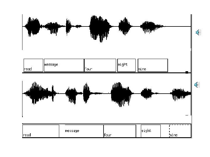
Pronunciation Example • Observations: 0/1
: – Problem: Phones can be pronounced differently • Speaker")
Acoustic Model • P(signal| phones): – Problem: Phones can be pronounced differently • Speaker differences, speaking rate, microphone • Phones may not even appear, different contexts – Observation sequence is uncertain • Solution: Hidden Markov Models – 1) Hidden => Observations uncertain – 2) Probability of word sequences => • State transition probabilities – 3) 1 st order Markov => use 1 prior state
![Acoustic Model • 3 -state phone model for [m] – Use Hidden Markov Model](http://slidetodoc.com/presentation_image_h2/3a4989b156cc1b7666ba216a0ac7f8b6/image-36.jpg "Acoustic Model • 3 -state phone model for [m] – Use Hidden Markov Model")
Acoustic Model • 3 -state phone model for [m] – Use Hidden Markov Model (HMM) 0. 3 0. 9 0. 4 Transition probabilities Onset 0. 7 Mid 0. 1 End 0. 6 Final C 3: C 1: C 2: 0. 3 0. 5 0. 2 C 5: C 3: C 4: 0. 1 0. 2 0. 7 C 6: C 4: C 6: 0. 4 0. 1 0. 5 Observation probabilities – Probability of sequence: sum of prob of paths

ASR Training • Models to train: – – Language model: typically tri-gram Observation likelihoods: B Transition probabilities: A Pronunciation lexicon: sub-phone, word • Training materials: – Speech files – word transcription – Large text corpus – Small phonetically transcribed speech corpus

Training • Language model: – Uses large text corpus to train n-grams • 500 M words • Pronunciation model: – HMM state graph – Manual coding from dictionary • Expand to triphone context and sub-phone models

HMM Training • Training the observations: – E. g. Gaussian: set uniform initial mean/variance • Train based on contents of small (e. g. 4 hr) phonetically labeled speech set (e. g. Switchboard) • Training A&B: – Forward-Backward algorithm training

Does it work? • Yes: – 99% on isolate single digits – 95% on restricted short utterances (air travel) – 80+% professional news broadcast • No: – 55% Conversational English – 35% Conversational Mandarin – ? ? Noisy cocktail parties
 are more likely than others – Given")
N-grams • Perspective: – Some sequences (words/chars) are more likely than others – Given sequence, can guess most likely next • Used in – Speech recognition – Spelling correction, – Augmentative communication – Other NL applications

Corpus Counts • Estimate probabilities by counts in large collections of text/speech • Issues: – Wordforms (surface) vs lemma (root) – Case? Punctuation? Disfluency? – Type (distinct words) vs Token (total)

Basic N-grams • Most trivial: 1/#tokens: too simple! • Standard unigram: frequency – # word occurrences/total corpus size • E. g. the=0. 07; rabbit = 0. 00001 – Too simple: no context! • Conditional probabilities of word sequences

Markov Assumptions • Exact computation requires too much data • Approximate probability given all prior wds – Assume finite history – Bigram: Probability of word given 1 previous • First-order Markov – Trigram: Probability of word given 2 previous • N-gram approximation Bigram sequence

Issues • Relative frequency – Typically compute count of sequence • Divide by prefix • Corpus sensitivity – Shakespeare vs Wall Street Journal • Very unnatural • Ngrams

Evaluating n-gram models • Entropy & Perplexity – Information theoretic measures – Measures information in grammar or fit to data – Conceptually, lower bound on # bits to encode • Entropy: H(X): X is a random var, p: prob fn – E. g. 8 things: number as code => 3 bits/trans – Alt. short code if high prob; longer if lower • Can reduce • Perplexity:

Entropy of a Sequence • Basic sequence • Entropy of language: infinite lengths – Assume stationary & ergodic

Cross-Entropy • Comparing models – Actual distribution unknown – Use simplified model to estimate • Closer match will have lower cross-entropy

Speech Recognition as Modern AI • Draws on wide range of AI techniques – Knowledge representation & manipulation • Optimal search: Viterbi decoding – Machine Learning • Baum-Welch for HMMs • Nearest neighbor & k-means clustering for signal id – Probabilistic reasoning/Bayes rule • Manage uncertainty in signal, phone, word mapping • Enables real world application
- Slides: 49