Hidden Markov Models Part 2 Algorithms CSE 4309

Hidden Markov Models Part 2: Algorithms CSE 4309 – Machine Learning Vassilis Athitsos Computer Science and Engineering Department University of Texas at Arlington 1

Hidden Markov Model • 2

The Basic HMM Problems • 3

The Basic HMM Problems • 4

Probability of Observations • 5

Probability of Observations • 6

Probability of Observations • 7

The Sum Rule • 8

The Sum Rule • 9

The Sum Rule • 10

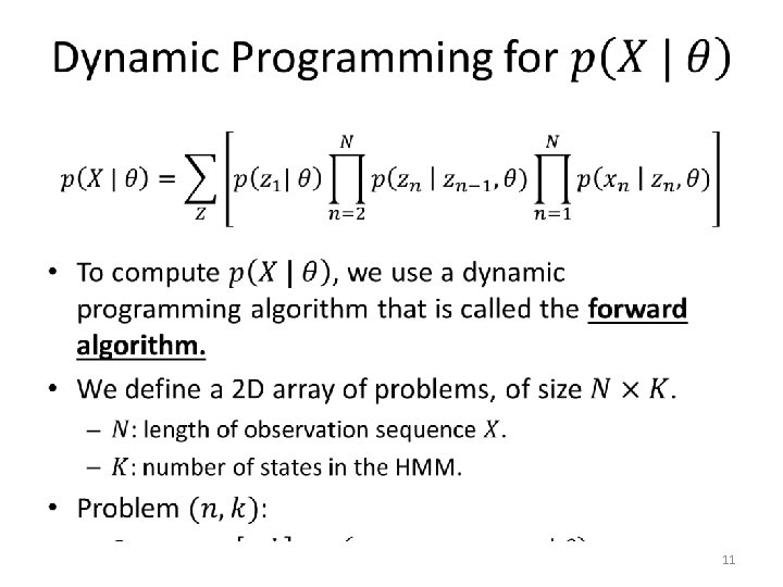
The Forward Algorithm - Initialization • 12

The Forward Algorithm - Initialization • 13

The Forward Algorithm - Initialization • 14

The Forward Algorithm - Main Loop • 15

The Forward Algorithm - Main Loop • 16

The Forward Algorithm - Main Loop • 17

The Forward Algorithm - Main Loop • 18

The Forward Algorithm • 19

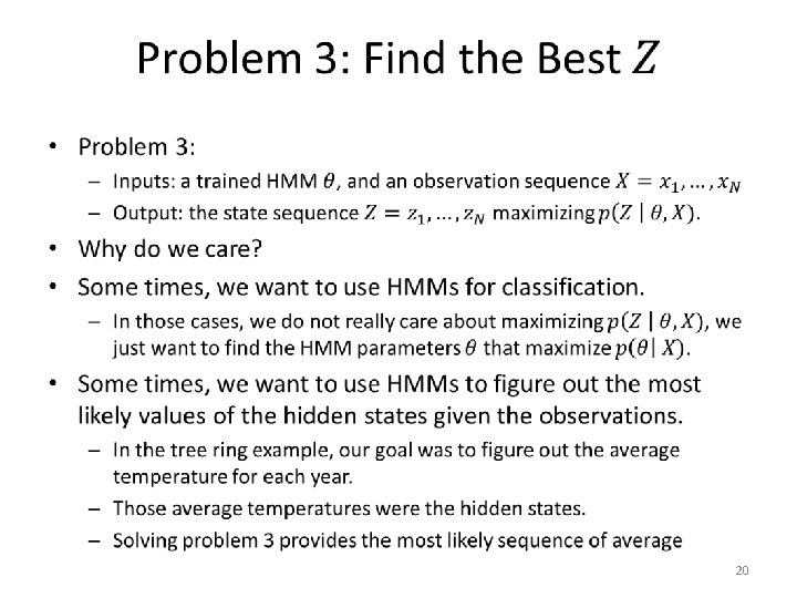
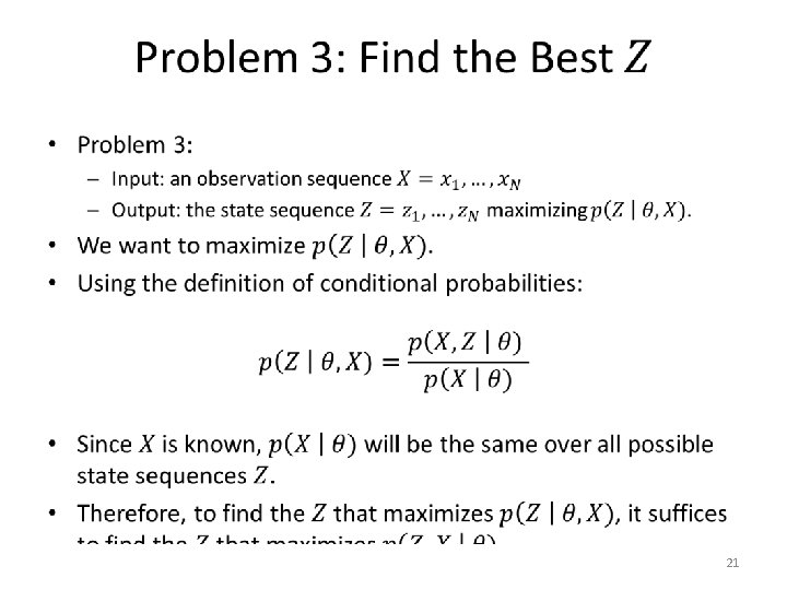
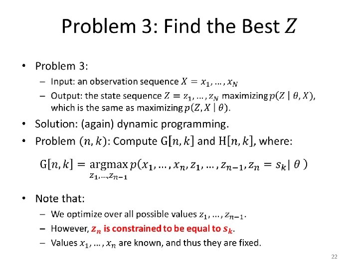
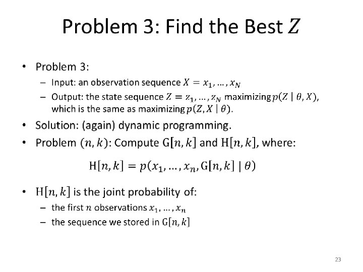
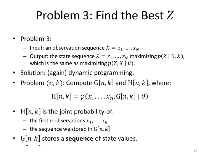
The Viterbi Algorithm • 25

The Viterbi Algorithm - Initialization • 26

The Viterbi Algorithm – Main Loop • 27

The Viterbi Algorithm – Main Loop • 28

The Viterbi Algorithm – Main Loop • 29

The Viterbi Algorithm – Output • 30

State Probabilities at Specific Times • 31

State Probabilities at Specific Times • 32

State Probabilities at Specific Times • 33

State Probabilities at Specific Times • 34

The Backward Algorithm • 35

Backward Algorithm - Initialization • 36

Backward Algorithm - Initialization • 37

Backward Algorithm - Initialization • 38

Backward Algorithm – Main Loop • 39

Backward Algorithm – Main Loop • We will take a closer look at the last step… 40

Backward Algorithm – Main Loop • 41

Backward Algorithm – Main Loop • 42

Backward Algorithm – Main Loop • 43

Backward Algorithm – Main Loop • 44

Backward Algorithm – Main Loop • 45

Backward Algorithm – Main Loop • 46

The Forward-Backward Algorithm • 47

Problem 1: Training an HMM • 48

Problem 1: Training an HMM • 49

Expectation-Maximization • When we wanted to learn a mixture of Gaussians, we had the following problem: – If we knew the probability of each object belonging to each Gaussian, we could estimate the parameters of each Gaussian. – If we knew the parameters of each Gaussian, we could estimate the probability of each object belonging to each Gaussian. – However, we know neither of these pieces of information. • The EM algorithm resolved this problem using: – An initialization of Gaussian parameters to some random or non-random values. – A main loop where: • The current values of the Gaussian parameters are used to estimate new weights of membership of every training object to every Gaussian. • The current estimated membership weights are used to estimate new parameters (mean and covariance matrix) for each Gaussian. 50

Expectation-Maximization • 51

Baum-Welch: Initialization • 52

Baum-Welch: Initialization • 53

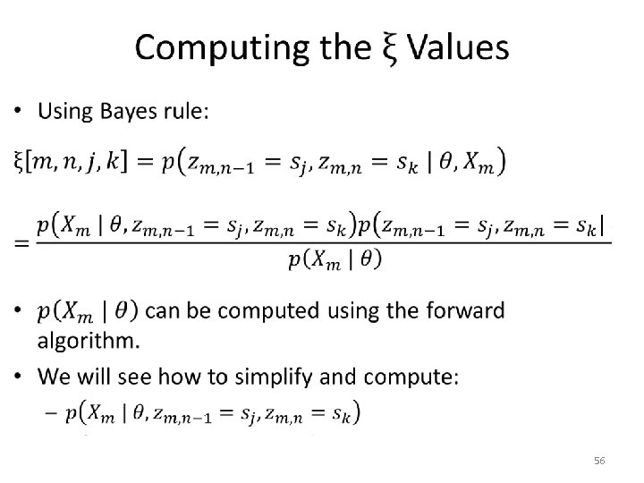
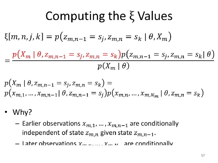
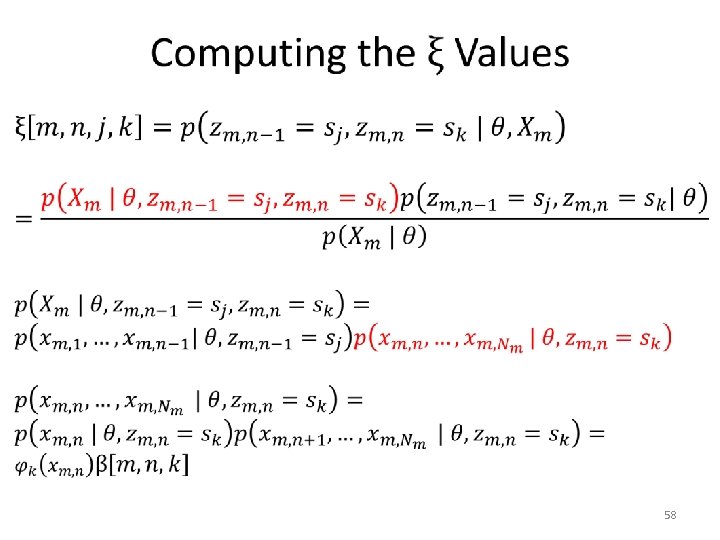
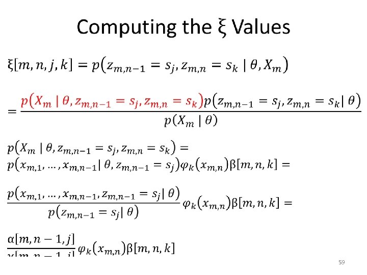
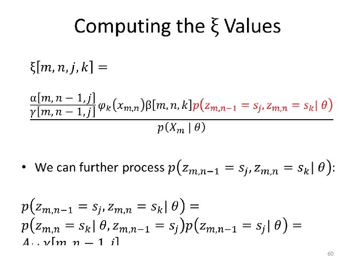
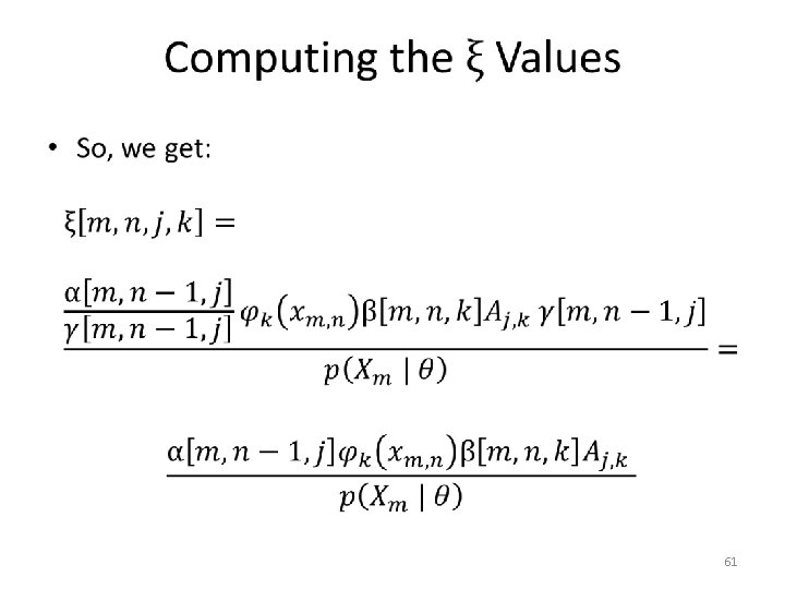
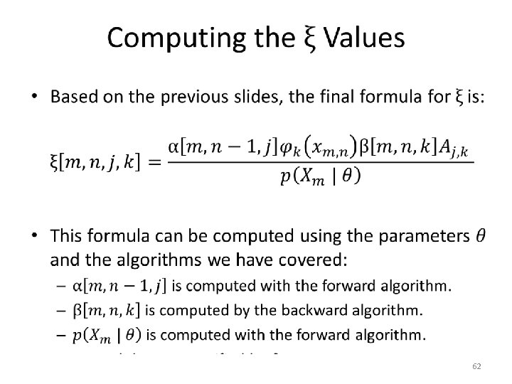
Baum-Welch: Expectation Step • 54

Baum-Welch: Expectation Step • 55

Baum-Welch: Summary of E Step • 63

Baum-Welch: Maximization Step • 64

Baum-Welch: Maximization Step • 65

Baum-Welch: Maximization Step • 66

Baum-Welch: Maximization Step • 67

Baum-Welch: Maximization Step • 68

Baum-Welch: Maximization Step • 69

Baum-Welch: Maximization Step • 70

Baum-Welch: Maximization Step • 71

Baum-Welch: Maximization Step • 72

Baum-Welch: Summary of M Step • 73

Baum-Welch: Summary of M Step • 74

Baum-Welch Summary • 75

Hidden Markov Models - Recap • 76

Hidden Markov Models - Recap • 77