Hidden Markov Models Markov chain property Probability of

Hidden Markov Models
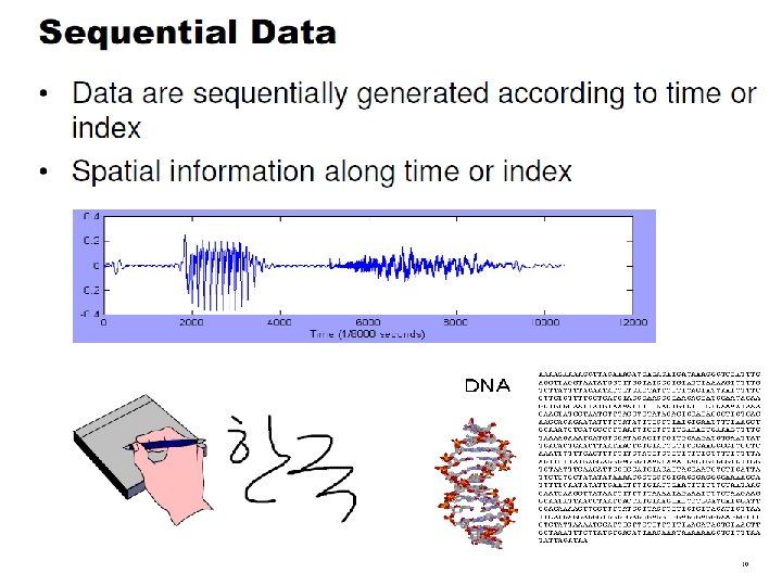
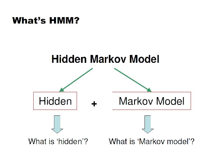

Markov chain property: • Probability of each subsequent state depends only on what was the previous state
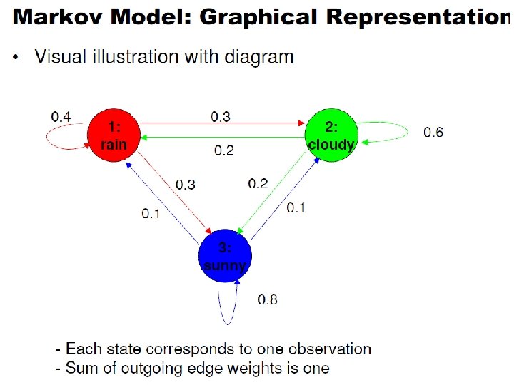

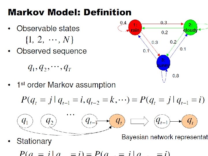
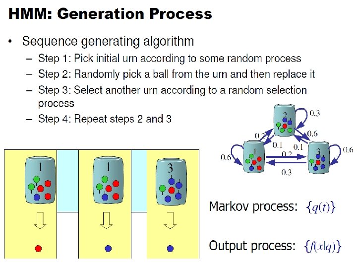
Markov Models • Set of states: • Process moves from one state to another generating a sequence of states : • Markov chain property: probability of each subsequent state depends only on what was the previous state: • To define Markov model, the following probabilities have to be specified: transition probabilities and initial probabilities • The output of the process is the set of states at each instant of time

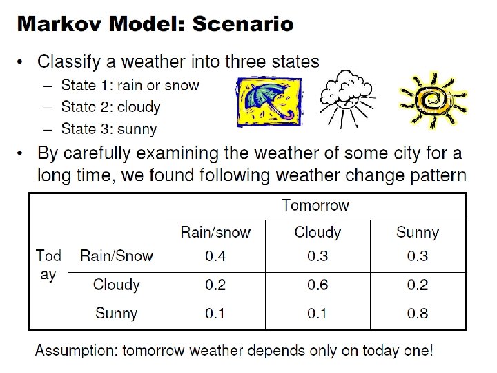
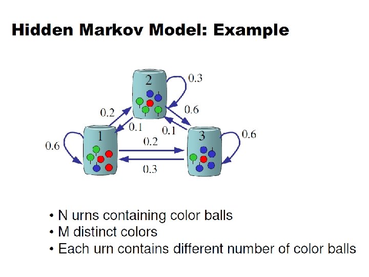
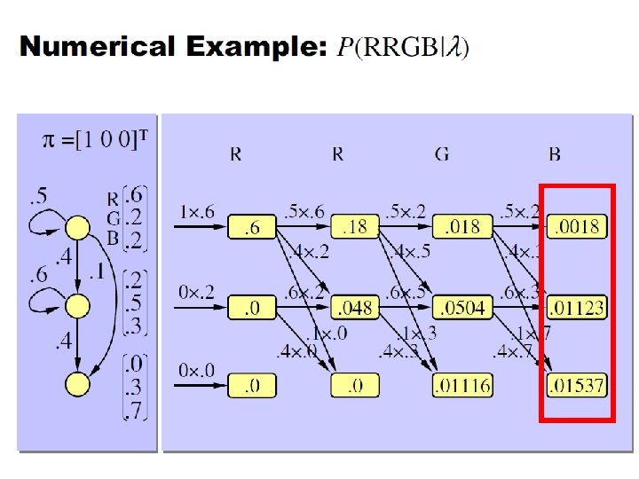
Example of Markov Model 0. 3 0. 7 Rain Dry 0. 2 0. 8 • Two states : ‘Rain’ and ‘Dry’. • Initial probabilities: say P(‘Rain’)=0. 4 , P(‘Dry’)=0. 6 • Suppose we want to calculate a probability of a sequence of states in our example, {‘Dry’, ’Rain’, Rain’}. P({‘Dry’, ’Rain’, Rain’} ) = ? ? .


Calculation of sequence probability • By Markov chain property, probability of state sequence can be found by the formula:


Markov Model to Hidden Markov Model

Markov Models State

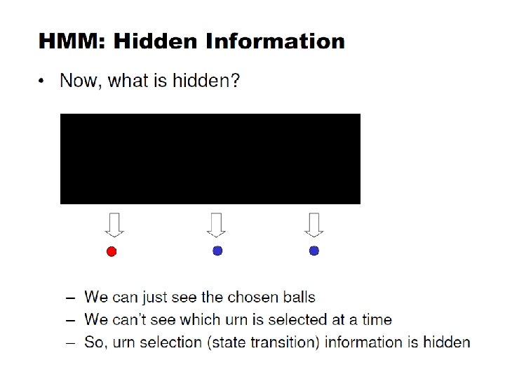
Hidden Markov Models • If you don’t have complete state information, but some observations at each state N - number of states : M - the number of observables: q 1 q 2 q 3 q 4 ……

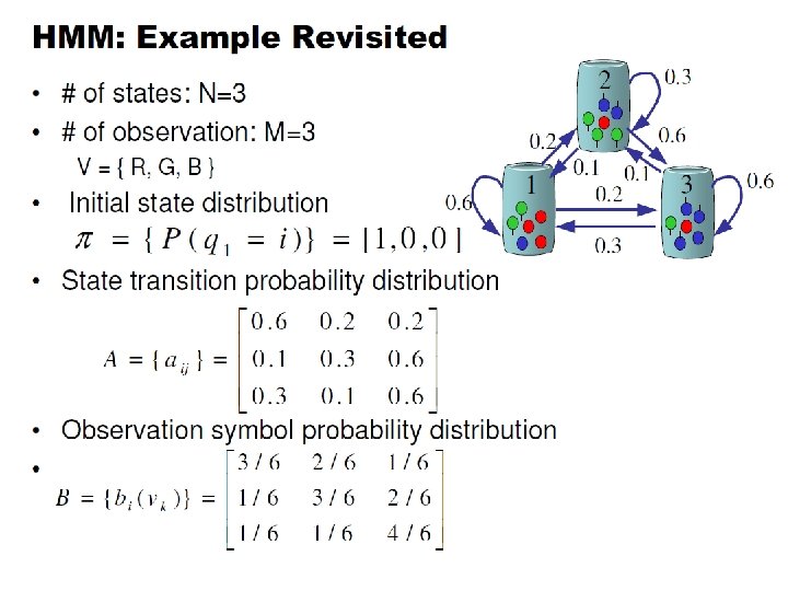
Hidden Markov Models State: { , , } Observable: { , 0. 1 0. 3 0. 9 0. 7 0. 8 0. 2 }
 = initial probabilities : =( i) ,")
Hidden Markov Models n M=(A, B, ) = initial probabilities : =( i) , i = P(si)

HMM Assumptions • Markov assumption: the state transition depends only on the origin and destination • Output-independent assumption: all observation frames are dependent on the state that generated them, not on neighbouring observation frames
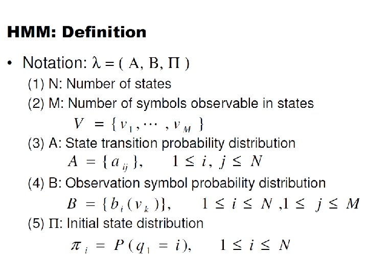
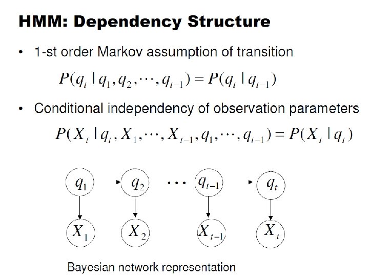

Hidden Markov models. • The observation is turned to be a probabilistic function (discrete or continuous) of a state instead of an one-to-one correspondence of a state • Each state randomly generates one of M observations (or visible states) • To define hidden Markov model, the following probabilities have to be specified: matrix of transition probabilities A=(aij), aij= P(si | sj) , matrix of observation probabilities B=(bi (vm )), bi(vm ) = P(vm | si) and a vector of initial probabilities =( i), i = P(si). Model is represented by M=(A, B, ).

HMM Formalism S S S K K K • {S, K, P, A, B} • S : {s 1…s. N } are the values for the hidden states • K : {k 1…k. M } are the values for the observations

HMM Formalism S A S B K • • A S B K K {S, K, P, A, B} P = { i} are the initial state probabilities A = {aij} are the state transition probabilities B = {bik} are the observation state probabilities K
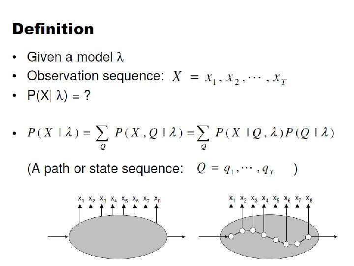
: Given the observation sequence O=o")
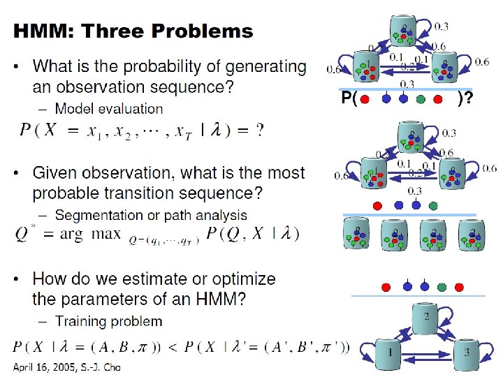
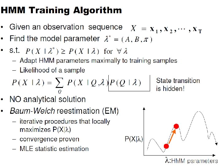
The Three Basic HMM Problems • Problem 1 (Evaluation): Given the observation sequence O=o 1, …, o. T and an HMM model how do we compute the probability of O given the model? • Problem 2 (Decoding): Given the observation sequence O=o 1, …, o. T and an HMM model , how do we find the state sequence that best explains the observations? Problem 3 (Learning): How do we adjust the model parameters , to maximize ?
")
Evaluation ( Model Fit)

Evaluation in an HMM • Compute the probability of a given observation sequence • Given an observation sequence, compute the most likely hidden state sequence • Given an observation sequence and set of possible models, which model most closely fits the data?
 – How can we compute likelihood of observations")
• MODEL FIT ( Evaluation) – How can we compute likelihood of observations and hidden states given known emission and transition probabilities? Compute: p(“Dog”/NOUN, ”is”/VERB, ”Good”/ADJ | {aij}, {bkm}) – How can we compute likelihood of observations given known emission and transition probabilities? p(“Dog”, ”is”, ”Good” | {aij}, {bkm})

Evaluation • Determine the probability that a particular sequence of symbols O was generated by that model

Forward recursion • Initialization: • Forward recursion: • Termination:

Backward recursion • Initialization: • Backward recursion: • Termination:

Decoding
 • How can we infer the sequence of hidden states")
• INFERENCE (Decoding) • How can we infer the sequence of hidden states given the observations and the known emission and transition probabilities? • Maximize: • p(“Dog”/? , ”is”/? , “Good”/? | {aij}, {bkm}) with respect to the unknown labels

Decoding n Given a set of symbols O determine the most likely sequence of hidden states Q that led to the observations We want to find the state sequence Q which maximizes P(Q|o 1, o 2, . . . , o. T)

Decoding o 1 ot-1 ot ot+1 Given an observation sequence and a model, compute the probability of the observation sequence o. T

Decoding x 1 xt-1 xt xt+1 x. T o 1 ot-1 ot ot+1 o. T

Decoding x 1 xt-1 xt xt+1 x. T o 1 ot-1 ot ot+1 o. T

Decoding x 1 xt-1 xt xt+1 x. T o 1 ot-1 ot ot+1 o. T

Decoding x 1 xt-1 xt xt+1 x. T o 1 ot-1 ot ot+1 o. T

Decoding x 1 xt-1 xt xt+1 x. T o 1 ot-1 ot ot+1 o. T

Forward Procedure x 1 xt-1 xt xt+1 x. T o 1 ot-1 ot ot+1 o. T • Special structure gives us an efficient solution using dynamic programming. • Intuition: Probability of the first t observations is the same for all possible t+1 length state sequences. • Define:

Forward Procedure x 1 xt-1 xt xt+1 x. T o 1 ot-1 ot ot+1 o. T

Forward Procedure x 1 xt-1 xt xt+1 x. T o 1 ot-1 ot ot+1 o. T

Forward Procedure x 1 xt-1 xt xt+1 x. T o 1 ot-1 ot ot+1 o. T

Forward Procedure x 1 xt-1 xt xt+1 x. T o 1 ot-1 ot ot+1 o. T

Forward Procedure x 1 xt-1 xt xt+1 x. T o 1 ot-1 ot ot+1 o. T

Forward Procedure x 1 xt-1 xt xt+1 x. T o 1 ot-1 ot ot+1 o. T

Forward Procedure x 1 xt-1 xt xt+1 x. T o 1 ot-1 ot ot+1 o. T

Forward Procedure x 1 xt-1 xt xt+1 x. T o 1 ot-1 ot ot+1 o. T

Backward Procedure x 1 xt-1 xt xt+1 x. T o 1 ot-1 ot ot+1 o. T Probability of the rest of the states given the first state

Decoding Solution x 1 xt-1 xt xt+1 x. T o 1 ot-1 ot ot+1 o. T Forward Procedure Backward Procedure Combination

Best State Sequence o 1 ot-1 ot ot+1 o. T • Find the state sequence that best explains the observations • Viterbi algorithm •

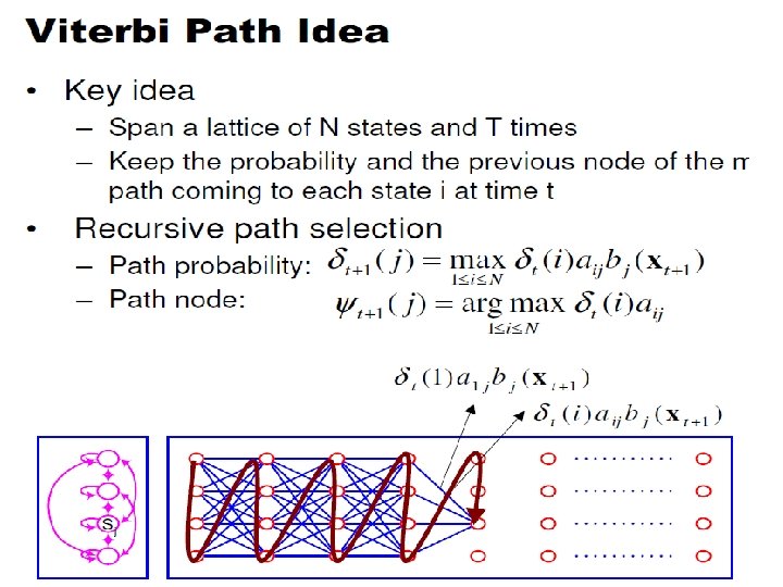
Viterbi algorithm qt-1 qt s 1 a 1 j si s. N aij a. Nj sj General idea: if best path ending in qt= sj goes through qt-1= si then it should coincide with best path ending in qt 1 = si

Viterbi Algorithm x 1 xt-1 j o 1 ot-1 ot ot+1 o. T The state sequence which maximizes the probability of seeing the observations to time t-1, landing in state j, and seeing the observation at time t

Viterbi Algorithm x 1 xt-1 xt xt+1 o 1 ot-1 ot ot+1 o. T Recursive Computation

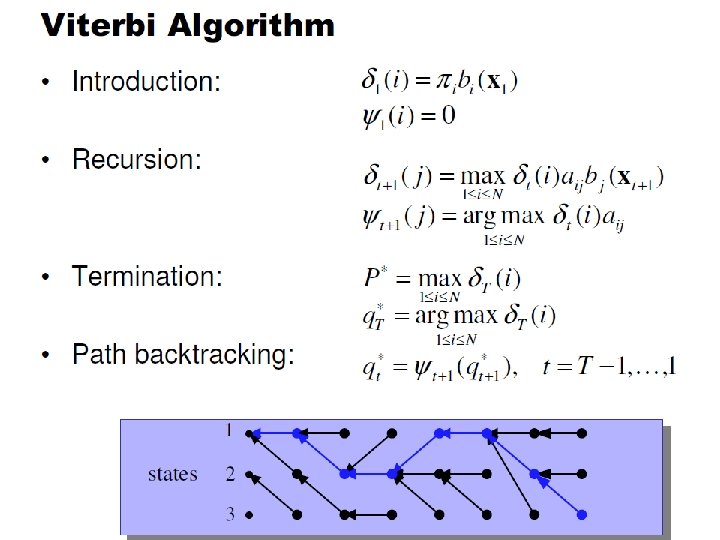
Viterbi algorithm n Initialization: n Forward recursion: n Termination:

Viterbi algorithm

Viterbi Algorithm x 1 xt-1 xt xt+1 x. T o 1 ot-1 ot ot+1 o. T Compute the most likely state sequence by working backwards

Learning

• LEARNING – How can we estimate the emission and transition probabilities given observations and assuming that hidden states are observable during learning process? – How can we estimate emission and transition probabilities given observations only?

Learning problem • Given a coarse structure of the model, determine HMM parameters M=(A, B, ) that best fit training data determine these parameters l l l
 as the probability of being in state")
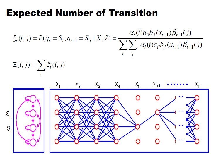
Baum-Welch algorithm n Define variable t(i, j) as the probability of being in state si at time t and in state sj at time t+1, given the observation sequence o 1, o 2, . . . , o. T
 as the probability of being in state si")
Baum-Welch algorithm • Define variable k(i) as the probability of being in state si at time t, given the observation sequence o 1, o 2 , . . . , o. T

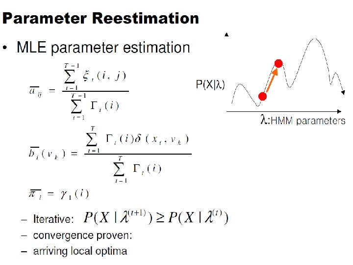
Parameter Estimation A B o 1 ot-1 A B ot ot+1 • Given an observation sequence, find the model that is most likely to produce that sequence. • No analytic method • Given a model and observation sequence, update the model parameters to better fit the observations. B o. T

Parameter Estimation A B o 1 ot-1 A B ot ot+1 B o. T Probability of traversing an arc Probability of being in state i

Parameter Estimation A B o 1 ot-1 A B ot+1 o. T Now we can compute the new estimates of the model parameters.

Applications

HMM Applications • Generating parameters for n-gram models • Tagging speech • Speech recognition

Example 1 -character recognition s 1 s 2 • The structure of hidden states: • Observation = number of islands in the vertical slice s 3

• Example 1 -character recognition After character image segmentation the following sequence of island numbers in 4 slices was observed : {1, 3, 2, 1}

Example 2 - face detection & recognition • The structure of hidden states:

Example 2 - face detection • A set of face images is used in the training of one HMM model N =6 states Image: 48, Training: 9, Correct detection: 90%, Pixels: 60 X 90

Example 2 - face recognition • Each individual in the database is represent by an HMM face model • A set of images representing different instances of same face are used to train each HMM N =6 states

Example 2 - face recognition Image: 400, Training : Half, Individual: 40, Pixels: 92 X 112

Extra slides

• HMM State-Emission Representation a 11=0. 7 K 1 b 11=0. 6 b 12=0. 1 1=1 K 2 • b 13=0. 3 S 1 K 3 a 12=0. 3 S 0 2=0 • a 21=0. 5 b 22=0. 7 b 23=0. 2 S 2 b 21=0. 1 a 22=0. 5 Note that sometimes a Hidden Markov Model is represented by having the emission arrows come off the arcs In this situation you would have a lot more emission arrows because there’s a lot more arcs… But the transition and emission probabilities are the same…it just takes longer to draw on your powerpoint presentation (self -conscious presentation)

HMM Notation State Sequence Variables: X 1, …, XT+1 Output Sequence Variables: O 1, …, OT Set of Hidden States (S 1, …, SN) Output Alphabet (K 1, …, KM) Initial State Probabilities ( 1, . . , N) i=p(X 1=Si), i=1, …, N • State Transition Probabilities (aij) i, j {1, …, N} • • • aij =p(Xt+1|Xt), t=1, …, T • Emission Probabilities (bij) i {1, …, N}, j {1, …, M} bij=p(Xt+1=Si|Xt=Sj), t=1, …, T
 and the O=o")
Evaluation Problem. • Evaluation problem. Given the HMM M=(A, B, ) and the O=o 1 o 2. . . o. T , calculate the probability that model M has generated sequence O. observation sequence • Direct Evaluation : Trying to find probability of observations O=o 1 o 2. . . o. T by means of considering all hidden state sequences • P(o 1 o 2. . . o. T ) = P(o 1 o 2. . . o. T , S ) {S is state sequence} • P(o 1 o 2. . . o. T ) = P(o 1 o 2. . . o. T /S ) P(S) • P(S) = • P(o 1 o 2. . . o. T /S ) = {Markov property} {Output independent assumption}

• NT hidden state sequences - exponential complexity. • Use Forward-Backward HMM algorithms for efficient calculations. • Define the forward variable k(i) as the joint probability of the partial observation sequence o 1 o 2. . . ok and that the hidden state at time k is si : k(i)= P(o 1 o 2. . . ok , qk= si )

The Trellis
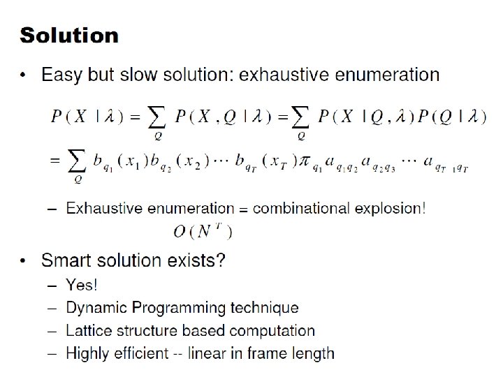

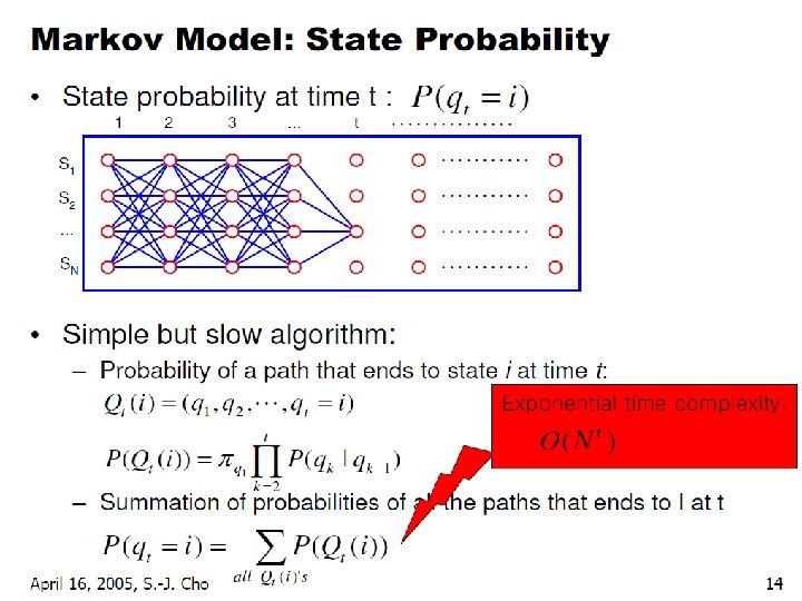
Problem 1: Probability of an Observation Sequence • What is ? • The probability of a observation sequence is the sum of the probabilities of all possible state sequences in the HMM. • Naïve computation is very expensive. Given T observations and N states, there are NT possible state sequences. • Even small HMMs, e. g. T=10 and N=10, contain 10 billion different paths • Solution to this and problem 2 is to use dynamic programming

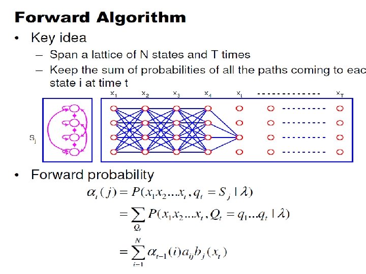
Forward Probabilities • What is the probability that, given an HMM , at time t the state is i and the partial observation o 1 … ot has been generated?

Forward Probabilities

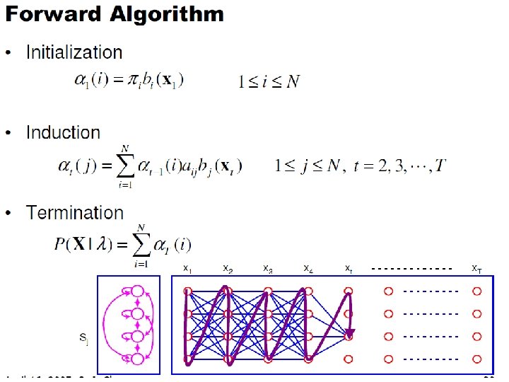
Forward Algorithm • Initialization: • Induction: • Termination:

Forward Algorithm Complexity • In the naïve approach to solving problem 1 it takes on the order of 2 T*NT computations • The forward algorithm takes on the order of N 2 T computations

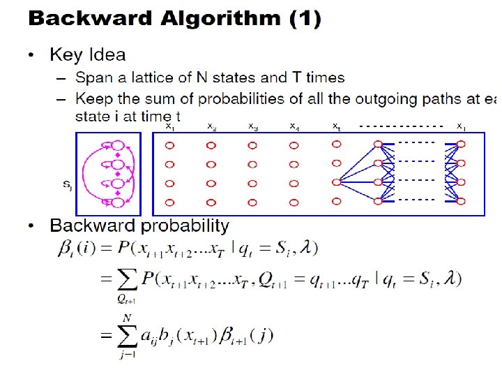
Backward Probabilities • Analogous to the forward probability, just in the other direction • What is the probability that given an HMM and given the state at time t is i, the partial observation ot+1 … o. T is generated?

Backward Probabilities

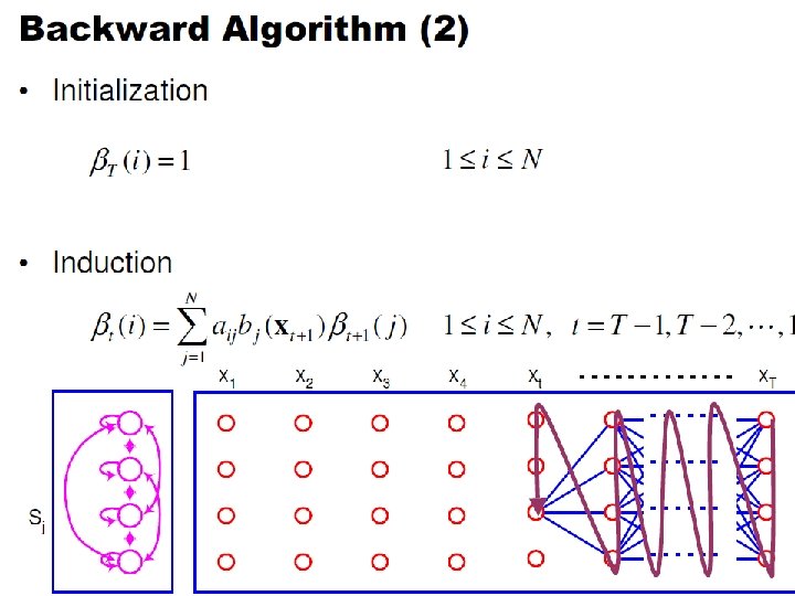
Backward Algorithm • Initialization: • Induction: • Termination:

Re-estimation of Emission Probabilities • Emission probabilities are re-estimated as • Formally: Where Note that here is the Kronecker delta function and is not related to the in the discussion of the Viterbi algorithm!!

The Updated Model • Coming from we get to by the following update rules:

Expectation Maximization • The forward-backward algorithm is an instance of the more general EM algorithm – The E Step: Compute the forward and backward probabilities for a give model – The M Step: Re-estimate the model parameters
 gives us the sum")
Problem 2: Decoding • The solution to Problem 1 (Evaluation) gives us the sum of all paths through an HMM efficiently. • For Problem 2, we wan to find the path with the highest probability. • We want to find the state sequence Q=q 1…q. T, such that

Viterbi Algorithm • Similar to computing the forward probabilities, but instead of summing over transitions from incoming states, compute the maximum • Forward: • Viterbi Recursion:

Viterbi Algorithm • Initialization: • Induction: • Termination: • Read out path:

Problem 3: Learning • Up to now we’ve assumed that we know the underlying model • Often these parameters are estimated on annotated training data, which has two drawbacks: – Annotation is difficult and/or expensive – Training data is different from the current data • We want to maximize the parameters with respect to the current data, i. e. , we’re looking for a model , such that

Problem 3: Learning • Unfortunately, there is no known way to analytically find a global maximum, i. e. , a model , such that • But it is possible to find a local maximum • Given an initial model , we can always find a model , such that
 algorithm, which is a hill-climbing algorithm")
Parameter Re-estimation • Use the forward-backward (or Baum-Welch) algorithm, which is a hill-climbing algorithm • Using an initial parameter instantiation, the forward-backward algorithm iteratively reestimates the parameters and improves the probability that given observation are generated by the new parameters

Parameter Re-estimation • Three parameters need to be re-estimated: – Initial state distribution: – Transition probabilities: ai, j – Emission probabilities: bi(ot)

Re-estimating Transition Probabilities • What’s the probability of being in state si at time t and going to state sj, given the current model and parameters?

Re-estimating Transition Probabilities

Re-estimating Transition Probabilities • The intuition behind the re-estimation equation for transition probabilities is • Formally:

Re-estimating Transition Probabilities • Defining As the probability of being in state si, given the complete observation O • We can say:

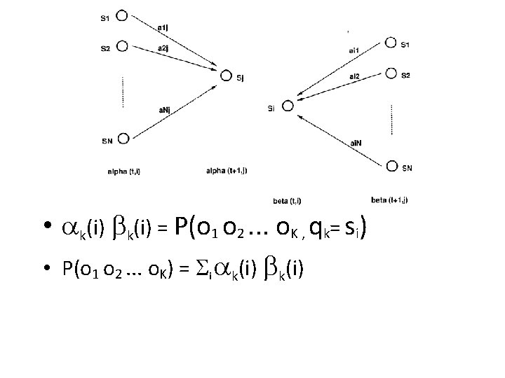
Review of Probabilities • Forward probability: The probability of being in state si, given the partial observation o 1, …, ot • Backward probability: The probability of being in state si, given the partial observation ot+1, …, o. T • Transition probability: The probability of going from state si, to state sj, given the complete observation o 1, …, o. T • State probability: The probability of being in state si, given the complete observation o 1, …, o. T

Re-estimating Initial State Probabilities • Initial state distribution: that si is a start state • Re-estimation is easy: • Formally: is the probability

Example of Hidden Markov Model 0. 3 0. 7 Low High 0. 2 0. 6 Rain 0. 4 0. 8 0. 4 0. 6 Dry

Example of Hidden Markov Model • Two states : ‘Low’ and ‘High’ atmospheric pressure. • Two observations : ‘Rain’ and ‘Dry’. • Transition probabilities: P(‘Low’|‘Low’)=0. 3 , P(‘High’|‘Low’)=0. 7 , P(‘Low’|‘High’)=0. 2, P(‘High’|‘High’)=0. 8 • Observation probabilities : P(‘Rain’|‘Low’)=0. 6 , P(‘Dry’|‘Low’)=0. 4 , P(‘Rain’|‘High’)=0. 4 , P(‘Dry’|‘High’)=0. 3. • Initial probabilities: say P(‘Low’)=0. 4 , P(‘High’)=0. 6.

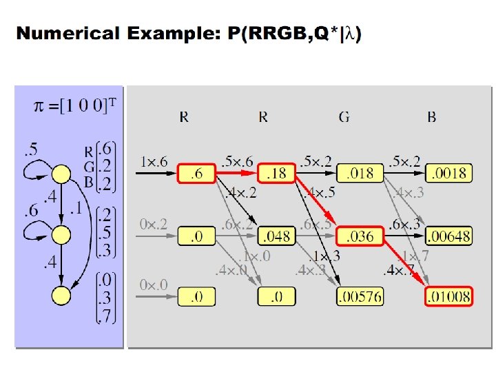
Calculation of observation sequence probability • Suppose we want to calculate a probability of a sequence of observations in our example, {‘Dry’, ’Rain’}. • Consider all possible hidden state sequences: P({‘Dry’, ’Rain’} ) = P({‘Dry’, ’Rain’} , {‘Low’, ’Low’}) + P({‘Dry’, ’Rain’} , {‘Low’, ’High’}) + P({‘Dry’, ’Rain’} , {‘High’, ’Low’}) + P({‘Dry’, ’Rain’} , {‘High’, ’High’}) where first term is : P({‘Dry’, ’Rain’} , {‘Low’, ’Low’})= P({‘Dry’, ’Rain’} | {‘Low’, ’Low’}) P({‘Low’, ’Low’}) = ? ?
 and the observation sequence O=o o.")
Main issues using HMMs : M=(A, B, ) and the observation sequence O=o o. . . o , calculate the probability that model M has generated sequence O. • Decoding problem. Given the HMM M=(A, B, ) and the observation sequence O=o o. . . o , calculate the most likely sequence of hidden states s that produced this observation sequence O. • Learning problem. Given some training observation sequences O=o o. . . o and general structure of HMM (numbers of hidden and visible states), adjust M=(A, B, ) to maximize the probability. O=o. . . o denotes a sequence of observations o {v , …, v }. Evaluation problem. Given the HMM 1 2 K i 1 1 K k 1 M 2 K
. • Typed word recognition, assume all characters are separated. • Character")
Word recognition example(1). • Typed word recognition, assume all characters are separated. • Character recognizer outputs probability of the image being particular character, P(image|character). a 0. 5 b 0. 03 c 0. 005 z 0. 31 Hidden state Observation
. • Hidden states of HMM = characters. • Observations = typed")
Word recognition example(2). • Hidden states of HMM = characters. • Observations = typed images of characters segmented from the image. Note that there is an infinite number of observations • Observation probabilities = character recognizer scores. • Transition probabilities will be defined differently in two subsequent models.
. • If lexicon is given, we can construct separate HMM models")
Word recognition example(3). • If lexicon is given, we can construct separate HMM models for each lexicon word. Amherst a m h e r s t Buffalo b u f f a l o 0. 5 0. 03 0. 4 0. 6 • Here recognition of word image is equivalent to the problem of evaluating few HMM models. • This is an application of Evaluation problem.
. • We can construct a single HMM for all words. •")
Word recognition example(4). • We can construct a single HMM for all words. • Hidden states = all characters in the alphabet. • Transition probabilities and initial probabilities are calculated from language model. • Observations and observation probabilities are as before. a m f r t o b h e s v • Here we have to determine the best sequence of hidden states, the one that most likely produced word image. • This is an application of Decoding problem.

= P(o 1 , q 1= si )")
Forward recursion for HMM • Initialization: 1(i)= P(o 1 , q 1= si ) = i bi (o 1) , 1<=i<=N. • Forward recursion: k+1(j)= P(o 1 o 2. . . ok+1 , qk+1= sj ) = i P(o 1 o 2. . . ok+1 , qk= si , qk+1= sj ) = i P(o 1 o 2. . . ok , qk= si) aij bj (ok+1 ) = [ i k(i) aij ] bj (ok+1 ) , 1<=j<=N, 1<=k<=K-1. • Termination: P(o 1 o 2. . . o. K) = i P(o 1 o 2. . . o. K , q. K= si) = i K(i) • Complexity : N 2 K operations.
 as the joint probability")
Backward recursion for HMM • Define the backward variable k(i) as the joint probability of the partial observation sequence ok+1 ok+2. . . o. K given that the hidden state at time k is si : k(i)= P(ok+1 ok+2. . . o. K |qk= si ) • Initialization: K(i)= 1 , 1<=i<=N. • Backward recursion: k(j)= P(ok+1 ok+2. . . o. K | qk= sj ) = i P(ok+1 ok+2. . . o. K , qk+1= si | qk= sj ) = i P(ok+2 ok+3. . . o. K | qk+1= si) aji bi (ok+1 ) = i k+1(i) aji bi (ok+1 ) , 1<=j<=N, 1<=k<=K-1. • Termination: P(o 1 o 2. . . o. K) = i P(o 1 o 2. . . o. K , q 1= si) = i P(o 1 o 2. . . o. K |q 1= si) P(q 1= si) = i 1(i) bi (o 1) i

Decoding problem • We want to find the state sequence Q= q 1…q. K which maximizes P(Q | o 1 o 2. . . o. K ) , or equivalently P(Q , o 1 o 2. . . o. K ). • Brute force consideration of all paths takes exponential time. Use efficient Viterbi algorithm instead. k(i) as the maximum probability of producing observation sequence o 1 o 2. . . ok when moving along any hidden state sequence q 1… qk-1 and getting into qk= si. k(i) = max P(q 1… qk-1 , qk= si , o 1 o 2. . . ok) where max is taken over all possible paths q 1… qk-1. • Define variable
 • General idea: if best path ending in qk= sj goes")
Viterbi algorithm (1) • General idea: if best path ending in qk= sj goes through qk-1= si then it should coincide with best path ending in qk-1= si. qk-1 s 1 si qk a 1 j aij a. Nj sj s. N • k(i) = max P(q 1… qk-1 , qk= sj , o 1 o 2. . . ok) = maxi [ aij bj (ok ) max P(q 1… qk-1= si , o 1 o 2. . . ok-1) ] • To backtrack best path keep info that predecessor of sj was si.
 • Initialization: 1(i) = max P(q 1= si , o 1)")
Viterbi algorithm (2) • Initialization: 1(i) = max P(q 1= si , o 1) = i bi (o 1) , 1<=i<=N. • Forward recursion: k(j) = max P(q 1… qk-1 , qk= sj , o 1 o 2. . . ok) = maxi [ aij bj (ok ) max P(q 1… qk-1= si , o 1 o 2. . . ok-1) ] = maxi [ aij bj (ok ) k-1(i) ] , 1<=j<=N, 2<=k<=K. • Termination: choose best path ending at time K maxi [ K(i) ] • Backtrack best path. This algorithm is similar to the forward recursion of evaluation problem, with replaced by max and additional backtracking.

Learning problem • The most difficult of the three problems, because there is no known analytical method that maximizes the joint probability of the training data • Solved by the Baum-Welch (known as forward backward) algorithm and EM (Expectation maximization) algorithm

Hidden Markov Models Richard Golden (following approach of Chapter 9 of Manning and Schutze, 2000) REVISION DATE: April 15 (Tuesday), 2003
 a 11=0. 7 1 S 1 a 12=0. 3 S")
VMM (Visible Markov Model) a 11=0. 7 1 S 1 a 12=0. 3 S 0 a 21=0. 5 2 S 2 a 22=0. 5
 Part 1 Follows directly")
Direct Calculation of Model Fit (note use of “Markov” Assumptions) Part 1 Follows directly from the definition of a conditional probability: p(o, x)=p(o|x)p(x) EXAMPLE: P(“Dog”/NOUN, ”is”/VERB, ”Good”/ADJ | {aij}, {bij}) = p(“Dog”, ”is”, ”Good”|NOUN, VERB, ADJ {aij}, {bij}) X p(NOUN, VERB, ADJ | aij}, {bij})
 Part 2")
Direct Calculation of Likelihood of Labeled Observations (note use of “Markov” Assumptions) Part 2 EXAMPLE: Compute p(“DOG”/NOUN, ”is”/VERB, ”good”/ADJ|{aij}, {bkm})

Graphical Algorithm Representation of Direct Calculation of Likelihood of Observations and Hidden States (not hard!) K 1 a 11=0. 7 1=1 b 11=0. 6 b 13=0. 3 S 1 K 2 K 3 a 12=0. 3 S 0 2=0 b 12=0. 1 a 21=0. 5 b 22=0. 7 Note that “good” is The name Of the dogj So it is a Noun! b 23=0. 2 S 2 a 22=0. 5 b 21=0. 1 The likelihood of a particular “labeled” sequence of observations (e. g. , p(“Dog”/NOUN, ”is”/VERB, ”Good”/NOUN|{aij}, {bkm})) may be computed Using the “direct calculation” method using following simple graphical algorithm. Specifically, p(K 3/S 1, K 2/S 2, K 1/S 1 |{aij}, {bkm}))= 1 b 13 a 12 b 22 a 21 b 11

Extension to case where the likelihood of the observations given parameters is needed (e. g. , p( “Dog”, ”is”, ”good” | {aij}, {bij}) KILLER EQUATION!!!!!
 • Assume 1 multiplication per")
Efficiency of Calculations is Important (e. g. , Model-Fit) • Assume 1 multiplication per microsecond • Assume N=1000 word vocabulary and T=7 word sentence. • (2 T+1)NT+1 multiplications by “direct calculation” yields (2(7)+1)(1000)(7+1) is about 475, 000 million years of computer time!!! • 2 N 2 T multiplications using “forward method” is about 14 seconds of computer time!!!

Forward, Backward, and Viterbi Calculations • Forward calculation methods are thus very useful. • Forward, Backward, and Viterbi Calculations will now be discussed.

Forward Calculations – Overview TIME 3 TIME 2 K 1 K 3 K 2 TIME 4 K 3 K 1 K 2 K 3 b 12=0. 1 b 11=0. 6 a 11=0. 7 S 1 1 b 13=0. 3 a 12=0. 3 S 1 a 21=0. 5 S 0 2 S 2 a 22=0. 5 b 21=0. 1 K 1 S 2 b 23=0. 2 b 22=0. 1 K 2 K 3 K 1 K 2 K 3
 TIME 2 K 1 K 2")
Forward Calculations – Time 2 (1 word example) TIME 2 K 1 K 2 NOTE: that 1 (2)+ 2 (2) is the likelihood of the observation/word “K 3” in this “ 1 word example” K 3 b 13=0. 3 a 11=0. 7 S 1 1 a 12=0. 3 S 1 a 21=0. 5 S 0 2 S 2 a 22=0. 5 b 23=0. 2 K 1 K 2 K 3 S 2
 TIME 3 TIME 2 K 1")
Forward Calculations – Time 3 (2 word example) TIME 3 TIME 2 K 1 K 3 K 2 TIME 4 K 3 b 12=0. 1 b 11=0. 6 a 11=0. 7 S 1 1 1(3) a 12=0. 3 S 1 a 21=0. 5 S 0 2 S 2 a 22=0. 5 b 21=0. 1 K 1 S 2 b 22=0. 1 K 2 K 3 K 1 K 2 K 3
 TIME 3 TIME 2 K 1")
Forward Calculations – Time 4 (3 word example) TIME 3 TIME 2 K 1 K 3 TIME 4 K 2 K 3 K 1 K 2 K 3 b 12=0. 1 b 13=0. 3 b 11=0. 6 a 11=0. 7 S 1 1 a 12=0. 3 S 1 S 1 a 21=0. 5 S 0 2 S 2 K 1 S 2 a 22=0. 5 b 21=0. 1 S 2 b 23=0. 2 b 22=0. 1 K 2 K 3 K 1 K 2 K 3
 1(t) 2(t) L(t) p(K 1… Kt)")
Forward Calculation of Likelihood Function (“emit and jump”) 1(t) 2(t) L(t) p(K 1… Kt) t=1 t=2 t=3 t=4 (0 -word) (1 -word) (2 -word) (3 -word) 1. 0 0. 21 0. 0462 1 =1 1(1) a 11 b 13 + 2(1) a 21 b 23 1(2)a 11 b 12 + 2(2)a 21 b 12 0. 021294 0. 09 0. 0378 0. 010206 2 =0 1(1) a 12 b 13 + 2(1) a 22 b 23 0. 084 1(3) + 2(3) 0. 0315 1(4) + 2(4) 1. 0 1(1) + 2(1) 0. 3 1(2) + 2(2)

Backward Calculations – Overview TIME 3 TIME 2 K 1 K 3 K 2 TIME 4 K 3 K 1 K 2 K 3 b 12=0. 1 b 11=0. 6 a 11=0. 7 S 1 1 b 13=0. 3 a 12=0. 3 S 1 a 21=0. 5 S 0 2 S 2 a 22=0. 5 b 21=0. 1 K 1 S 2 b 23=0. 2 b 22=0. 1 K 2 K 3 K 1 K 2 K 3

Backward Calculations – Time 4 TIME 4 K 1 K 2 K 3 b 11`=0. 6 S 1 S 2 b 21=0. 1

Backward Calculations – Time 3 TIME 3 K 1 K 2 K 3 b 11`=0. 6 S 1 S 2 b 21=0. 1
+ 2")
Backward Calculations – Time 2 TIME 3 TIME 2 NOTE: that 1 (2)+ 2 (2) is the likelihood the observation/word sequence “K 2, K 1” in this “ 2 word example” K 1 K 2 TIME 4 K 3 K 1 K 2 K 3 b 12=0. 1 S 1 b 13=0. 3 a 11=0. 7 a 12=0. 3 S 1 a 21=0. 5 a 22=0. 5 S 2 b 23=0. 2 b 22=0. 7 K 1 K 2 K 3

Backward Calculations – Time 1 TIME 3 TIME 2 K 1 K 3 K 2 TIME 4 K 3 K 1 K 2 K 3 b 12=0. 1 b 11=0. 6 a 11=0. 7 S 1 1 b 13=0. 3 a 12=0. 3 S 1 a 21=0. 5 S 0 2 S 2 a 22=0. 5 b 21=0. 1 K 1 S 2 b 23=0. 2 b 22=0. 1 K 2 K 3 K 1 K 2 K 3
 t=1 t=2 t=3 t=4 1(t) 0.")
Backward Calculation of Likelihood Function (“EMIT AND JUMP”) t=1 t=2 t=3 t=4 1(t) 0. 0315 0. 045 0. 6 1 a 11 b 11 1(1) + + a 12 b 21 1(1) b 11 2(t) 0. 029 0. 245 0. 1 a 11 b 11 1(1) + + a 12 b 21 1(1) b 21 L(t) 0. 0315 1 1(1) + 2 2(1) 0. 290 1(2) + 2(2) 0. 7 1(3) + 2(3) p(Kt… KT) 1 1
 1. 0")
You get same answer going forward or backward!! Backward Forward t=1 1(t) 1. 0 1 =1 2(t) 0. 0 2 =0 L(t) p(K 1… Kt ) 1. 0 1(1) + 2(1) t=2 t=3 t=4 0. 21 1(1) a 11 b 13 + 2(1) a 21 b 23 0. 0462 1(2)a 11 b 12 + 2(2)a 21 b 12 0. 021294 0. 09 1(1) a 12 b 13 + 2(1) a 22 b 23 0. 0378 0. 010206 0. 3 1(2) + 2(2) 0. 084 1(3) + 2(3) 0. 0315 1(4) + 2(4) t=1 t=2 t=3 t=4 1(t) 0. 0315 0. 045 a 11 b 11 1(1) + + a 12 b 21 1(1) 0. 6 b 11 1 2(t) 0. 029 0. 245 a 11 b 11 1(1) + + a 12 b 21 1(1) 0. 1 b 21 1 L(t) p(Kt… KT ) 0. 0315 0. 290 1(2) + 2(2) 0. 7 1(3) + 2(3) 1 1 1(1) + 2 2(1)

The Forward-Backward Method • Note the forward method computes: • Note the backward method computes (t>1): • We can do the forward-backward method which computes p(K 1, …, KT) using formula (using any choice of t=1, …, T+1!):
 t=1 t=2 t=3 t=4 1. 0 0. 21")
Example Forward-Backward Calculation! Backward Forward 1(t) t=1 t=2 t=3 t=4 1. 0 0. 21 1(1) a 11 b 13 + 2(1) a 21 b 23 0. 0462 1(2)a 11 b 12 + 2(2)a 21 b 12 0. 021294 0. 09 1(1) a 12 b 13 + 2(1) a 22 b 23 0. 0378 0. 010206 0. 3 1(2) + 2(2) 0. 084 1(3) + 2(3) 1 =1 2(t) 0. 0 2 =0 L(t) p(K 1… Kt ) 1. 0 1(1) + 2(1) 0. 0315 1(4) + 2(4) t=1 t=2 t=3 t=4 1(t) 0. 0315 0. 045 a 11 b 11 1(1) + + a 12 b 21 1(1) 0. 6 b 11 1 2(t) 0. 029 0. 245 a 11 b 11 1(1) + + a 12 b 21 1(1) 0. 1 b 21 1 L(t) p(Kt… KT ) 0. 0315 0. 290 1(2) + 2(2) 0. 7 1(3) + 2(3) 1 1 1(1) + 2 2(1)

Solution to Problem 1 • The “hard part” of the 1 st Problem was to find the likelihood of the observations for an HMM • We can now do this using either the forward, backward, or forward-backward method.
 • Consider direct calculation")
Solution to Problem 2: Viterbi Algorithm (Computing “Most Probable” Labeling) • Consider direct calculation of labeled observations EXAMPLE: Compute p(“DOG”/NOUN, ”is”/VERB, ”good”/ADJ|{aij}, {bkm}) • Previously we summed these likelihoods together across all possible labelings to solve the first problem which was to compute the likelihood of the observations given the parameters (Hard part of HMM Question 1!). – We solved this problem using forward or backward method. • Now we want to compute all possible labelings and their respective likelihoods and pick the labeling which is the largest!
 • Just")
Efficiency of Calculations is Important (e. g. , Most Likely Labeling Problem) • Just as in the forward-backward calculations we can solve problem of computing likelihood of every possible one of the NT labelings efficiently • Instead of millions of years of computing time we can solve the problem in several seconds!!
 TIME 3 TIME 2 K")
Viterbi Algorithm – Overview (same setup as forward algorithm) TIME 3 TIME 2 K 1 K 3 K 2 TIME 4 K 3 K 1 K 2 K 3 b 12=0. 1 b 11=0. 6 a 11=0. 7 S 1 1 b 13=0. 3 a 12=0. 3 S 1 a 21=0. 5 S 0 2 S 2 a 22=0. 5 b 21=0. 1 K 1 S 2 b 23=0. 2 b 22=0. 1 K 2 K 3 K 1 K 2 K 3
 TIME 2 K 1 K 2")
Forward Calculations – Time 2 (1 word example) TIME 2 K 1 K 2 K 3 b 13=0. 3 1=1 a 11=0. 7 S 1 a 12=0. 3 S 1 a 21=0. 5 S 0 2=0 S 2 a 22=0. 5 b 23=0. 2 K 1 K 2 K 3 S 2
 TIME 2 K 1 K 2 K")
Backtracking – Time 2 (1 word example) TIME 2 K 1 K 2 K 3 b 13=0. 3 1=1 a 11=0. 7 S 1 a 12=0. 3 S 1 a 21=0. 5 S 0 2=0 S 2 a 22=0. 5 b 23=0. 2 K 1 K 2 K 3 S 2
 TIME 3 TIME 2 K 1 K 2")
Forward Calculations – (2 word example) TIME 3 TIME 2 K 1 K 2 K 3 K 1 K 2 TIME 4 K 3 b 12=0. 1 b 13=0. 3 S 1 1 S 1 a 11=0. 7 a 21=0. 5 a 12=0. 3 S 0 2 S 2 b 23=0. 2 K 1 K 2 K 3 a 22=0. 5 S 2 b 22=0. 1 K 2 K 3
 TIME 3 TIME 2 K 1 K 2 K")
BACKTRACKING – (2 word example) TIME 3 TIME 2 K 1 K 2 K 3 K 1 K 2 TIME 4 K 3 b 12=0. 1 b 13=0. 3 S 1 1 S 1 a 11=0. 7 a 21=0. 5 a 12=0. 3 S 0 2 S 2 b 23=0. 2 K 1 K 2 K 3 a 22=0. 5 S 2 b 22=0. 1 K 2 K 3

Formal Analysis of 2 word case
 TIME 3 TIME 2 K 1")
Forward Calculations – Time 4 (3 word example) TIME 3 TIME 2 K 1 K 3 TIME 4 K 2 K 3 K 1 K 2 K 3 b 12=0. 1 b 13=0. 3 b 11=0. 6 a 11=0. 7 S 1 1 a 12=0. 3 S 1 S 1 a 21=0. 5 S 0 2 S 2 K 1 S 2 a 22=0. 5 b 21=0. 1 S 2 b 23=0. 2 b 22=0. 1 K 2 K 3 K 1 K 2 K 3

Backtracking to Obtain Labeling for 3 word case TIME 3 TIME 2 K 1 K 3 TIME 4 K 2 K 3 K 1 K 2 K 3 b 12=0. 1 b 13=0. 3 b 11=0. 6 a 11=0. 7 S 1 1 a 12=0. 3 S 1 S 1 a 21=0. 5 S 0 2 S 2 K 1 S 2 a 22=0. 5 b 21=0. 1 S 2 b 23=0. 2 b 22=0. 1 K 2 K 3 K 1 K 2 K 3

Formal Analysis of 3 word case

Third Fundamental Question: Parameter Estimation • Make Initial Guess for {aij} and {bkm} • Compute probability one hidden state follows another given: {aij} and {bkm} and sequence of observations. (computed using forward-backward algorithm) • Compute probability of observed state given a hidden state given: {aij} and {bkm} and sequence of observations. (computed using forward-backward algorithm) • Use these computed probabilities to make an improved guess for {aij} and {bkm} • Repeat this process until convergence • Can be shown that this algorithm does in fact converge to correct choice for {aij} and {bkm} assuming that the initial guess was close enough. .
- Slides: 186