Hidden Markov Models A Hidden Markov Model consists

Hidden Markov Models

A Hidden Markov Model consists of 1. A sequence of states {Xt|t T} = {X 1, X 2, . . . , XT} , and 2. A sequence of observations {Yt |t T} = {Y 1, Y 2, . . . , YT}

• The sequence of states {X 1, X 2, . . . , XT} form a Markov chain moving amongst the M states {1, 2, …, M}. • The observation Yt comes from a distribution that is determined by the current state of the process Xt. (or possibly past observations and past states). • The states, {X 1, X 2, . . . , XT}, are unobserved (hence hidden).

Y 1 Y 2 Y 3 X 1 X 2 X 3 YT … The Hidden Markov Model XT

Some basic problems: from the observations {Y 1, Y 2, . . . , YT} 1. Determine the sequence of states {X 1, X 2, . . . , XT}. 2. Determine (or estimate) the parameters of the stochastic process that is generating the states and the observations. ;

Examples

Example 1 • A person is rolling two sets of dice (one is balanced, the other is unbalanced). He switches between the two sets of dice using a Markov transition matrix. • The states are the dice. • The observations are the numbers rolled each time.

Balanced Dice

Unbalanced Dice

Example 2 • The Markov chain is two state. • The observations (given the states) are independent Normal. • Both mean and variance dependent on state. HMM AR. xls

Example 3 –Dow Jones

Daily Changes Dow Jones

Hidden Markov Model? ?

Bear and Bull Market?

Speech Recognition • When a word is spoken the vocalization process goes through a sequence of states. • The sound produced is relatively constant when the process remains in the same state. • Recognizing the sequence of states and the duration of each state allows one to recognize the word being spoken.

• The interval of time when the word is spoken is broken into small (possibly overlapping) subintervals. • In each subinterval one measures the amplitudes of various frequencies in the sound. (Using Fourier analysis). The vector of amplitudes Yt is assumed to have a multivariate normal distribution in each state with the mean vector and covariance matrix being state dependent.

Hidden Markov Models for Biological Sequence Consider the Motif: [AT][CG][ACGT]*A[TG][GC] Some realizations: A C A G T C A A C C A G A - - A T T A T - A G - A T

Hidden Markov model of the same motif : [AT][CG][ACGT]*A[TG][GC] . 4 A. 2 C. 4 G. 2 T. 2. 6 A. 8 C G T. 2 1. 0 A C. 8 G. 2 T 1. 0 A. 8 C. 2 G T . 6 . 4 A C 1. 0 G T 1. 0 A C G. 2 T. 8 1. 0 A C. 8 G. 2 T

Profile HMMs Begin End

Computing Likelihood Let pij = P[Xt+1 = j|Xt = i] and P = (pij) = the M M transition matrix. Let = P[X 1 = i] and = the initial distribution over the states.

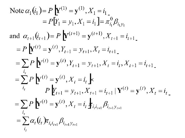
Now assume that P[Yt = yt |X 1 = i 1, X 2 = i 2, . . . , Xt = it] = P[Yt = yt | Xt = it] = p(yt| ) = Then P[X 1 = i 1, X 2 = i 2. . , XT = i. T, Y 1 = y 1, Y 2 = y 2, . . . , YT = y. T] = P[X = i, Y = y] =

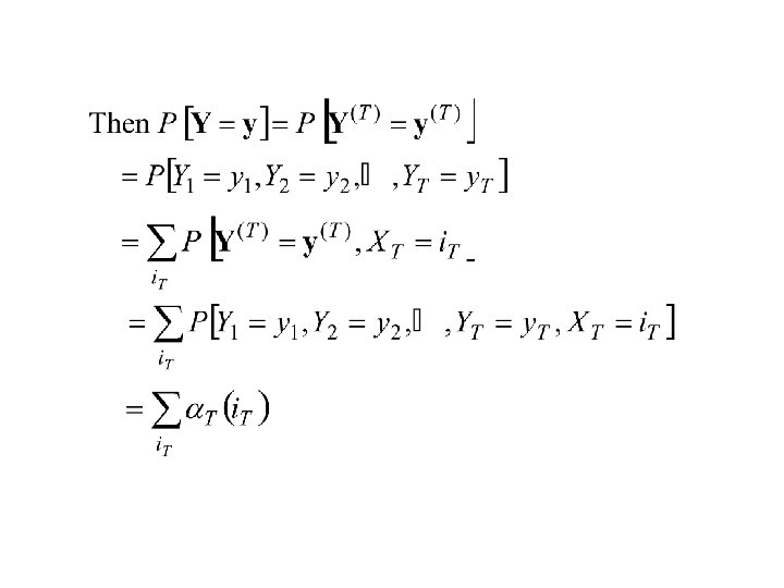
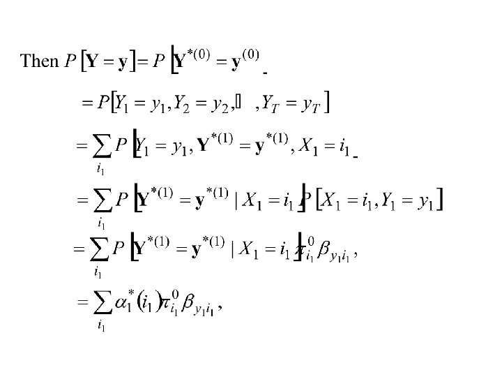
Therefore P[Y 1 = y 1, Y 2 = y 2, . . . , YT = y. T] = P[Y = y]

In the case when Y 1, Y 2, . . . , YT are continuous random variables or continuous random vectors, Let f(y| ) denote the conditional distribution of Yt given Xt = i. Then the joint density of Y 1, Y 2, . . . , YT is given by = f(y 1, y 2, . . . , y. T) = f(y) where = f(yt| )

Efficient Methods for computing Likelihood The Forward Method Consider

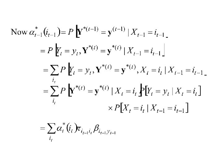
The Backward Procedure

Prediction of states from the observations and the model:

The Viterbi Algorithm (Viterbi Paths) Suppose that we know the parameters of the Hidden Markov Model. Suppose in addition suppose that we have observed the sequence of observations Y 1, Y 2, . . . , YT. Now consider determining the sequence of States X 1, X 2, . . . , XT.

Recall that P[X 1 = i 1, . . . , XT = i. T, Y 1 = y 1, . . . , YT = y. T] = P[X = i, Y = y] = Consider the problem of determining the sequence of states, i 1, i 2, . . . , i. T , that maximizes the above probability. This is equivalent to maximizing P[X = i|Y = y] = P[X = i, Y = y] / P[Y = y]

The Viterbi Algorithm We want to maximize P[X = i, Y = y] = Equivalently we want to minimize U(i 1, i 2, . . . , i. T) Where U(i 1, i 2, . . . , i. T) = -ln (P[X = i, Y = y]) =

• Minimization of U(i 1, i 2, . . . , i. T) can be achieved by Dynamic Programming. • This can be thought of as finding the shortest distance through the following grid of points. • By starting at the unique point in stage 0 and moving from a point in stage t to a point in stage t+1 in an optimal way. The distances between points in stage t and points in stage t+1 are equal to:

Dynamic Programming . . . Stage 0 Stage 1 Stage 2 Stage T-1 Stage T

• By starting at the unique point in stage 0 and moving from a point in stage t to a point in stage t+1 in an optimal way. • The distances between points in stage t and points in stage t+1 are equal to:

Dynamic Programming . . . Stage 0 Stage 1 Stage 2 Stage T-1 Stage T

Dynamic Programming . . . Stage 0 Stage 1 Stage 2 Stage T-1 Stage T

Let Then i 1 = 1, 2, …, M and it+1 = 1, 2, …, M; t = 1, …, T-2

Finally

Summary of calculations of Viterbi Path 1. i 1 = 1, 2, …, M 2. it+1 = 1, 2, …, M; t = 1, …, T-2 3.

An alternative approach to prediction of states from the observations and the model: It can be shown that:

Forward Probabilities 1. 2.

Backward Probabilities 1. 2. HMM generator (normal). xls

Estimation of Parameters of a Hidden Markov Model If both the sequence of observations Y 1, Y 2, . . . , YT and the sequence of States X 1, X 2, . . . , XT is observed Y 1 = y 1, Y 2 = y 2, . . . , YT = y. T, X 1 = i 1, X 2 = i 2, . . . , XT = i. T, then the Likelihood is given by:

the log-Likelihood is given by:

In this case the Maximum Likelihood estimates are: = the MLE of qi computed from the observations yt where Xt = i.

MLE (states unknown) If only the sequence of observations Y 1 = y 1, Y 2 = y 2, . . . , YT = y. T are observed then the Likelihood is given by:

• • It is difficult to find the Maximum Likelihood Estimates directly from the Likelihood function. The Techniques that are used are 1. The Segmental K-means Algorithm 2. The Baum-Welch (E-M) Algorithm

The Segmental K-means Algorithm In this method the parameters adjusted to maximize where is the Viterbi path are

Consider this with the special case Case: The observations {Y 1, Y 2, . . . , YT} are continuous Multivariate Normal with mean vector and covariance matrix when , i. e.

1. Pick arbitrarily M centroids a 1, a 2, … a. M. Assign each of the T observations yt (k. T if multiple realizations are observed) to a state it by determining : 2. Then

3. And 4. Calculate the Viterbi path (i 1, i 2, …, i. T) based on the parameters of step 2 and 3. 5. If there is a change in the sequence (i 1, i 2, …, i. T) repeat steps 2 to 4.

The Baum-Welch (E-M) Algorithm • The E-M algorithm was designed originally to handle “Missing observations”. • In this case the missing observations are the states {X 1, X 2, . . . , XT}. • Assuming a model, the states are estimated by finding their expected values under this model. (The E part of the E-M algorithm).

• With these values the model is estimated by Maximum Likelihood Estimation (The M part of the E-M algorithm). • The process is repeated until the estimated model converges.

The E-M Algorithm Let distribution of Y, X. Consider the function: denote the joint Starting with an initial estimate of. A sequence of estimates are formed by finding to maximize with respect to.

The sequence of estimates converge to a local maximum of the likelihood.

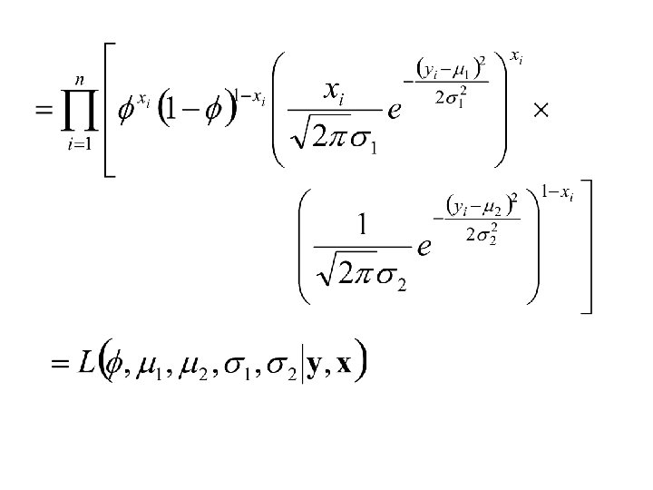
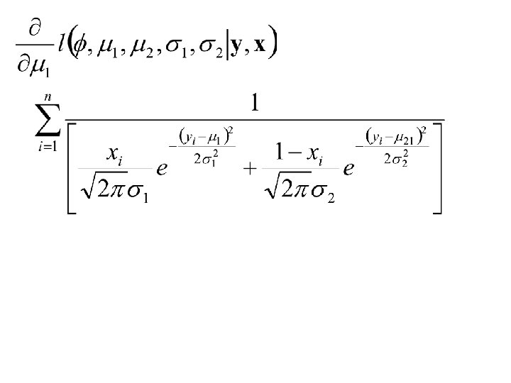
Example: Sampling from Mixtures Let y 1, y 2, …, yn denote a sample from the density: where and

Suppose that m = 2 and let x 1, x 2, …, x 1 denote independent random variables taking on the value 1 with probability f and 0 with probability 1 - f. Suppose that yi comes from the density We will also assume that g(y|qi) is normal with mean miand standard deviation si.

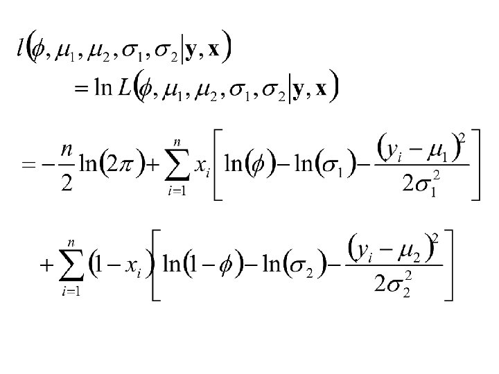
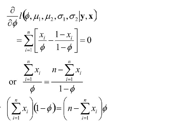
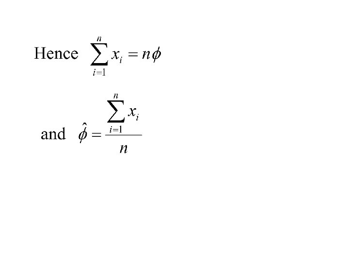
Thus the joint distribution of x 1, x 2, …, xn and let y 1, y 2, …, yn is:

In the case of an HMM the log-Likelihood is given by:

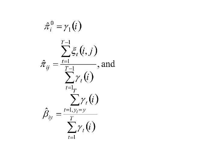
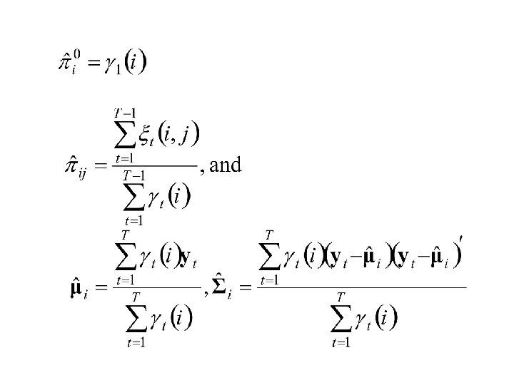
Recall and Expected no. of transitions from state i.

Let Expected no. of transitions from state i to state j.

The E-M Re-estimation Formulae Case 1: The observations {Y 1, Y 2, . . . , YT} are discrete with K possible values and

Case 2: The observations {Y 1, Y 2, . . . , YT} are continuous Multivariate Normal with mean vector and covariance matrix when , i. e.

Measuring distance between two HMM’s Let and denote the parameters of two different HMM models. We now consider defining a distance between these two models.

The Kullback-Leibler distance Consider the two discrete distributions and ( and in the continuous case) then define

and in the continuous case:

These measures of distance between the two distributions are not symmetric but can be made symmetric by the following:

In the case of a Hidden Markov model. where The computation of formidable in this case is

Juang and Rabiner distance Let denote a sequence of observations generated from the HMM with parameters: Let denote the optimal (Viterbi) sequence of states assuming HMM model.

Then define: and