Hidden Markov Models 1 2 K Lecture 4

Hidden Markov Models 1 2 K … Lecture 4, Thursday April 10, 2003

Outline • Hidden Markov Models – Formalism • The Three Basic Problems of HMMs • Solutions • Applications of HMMs for Automatic Speech Recognition (ASR) Lecture 4, Thursday April 10, 2003

Example: The Dishonest Casino A casino has two dice: • Fair die P(1) = P(2) = P(3) = P(4) = P(5) = P(6) = 1/6 • Loaded die P(1) = P(2) = P(3) = P(4) = P(5) = 1/10 P(6) = 1/2 Casino player switches back-&-forth between fair and loaded die once in a while Game: 1. You bet $1 2. You roll (always with a fair die) 3. Casino player rolls (maybe with fair die, maybe with loaded die) 4. Highest number wins $2 Lecture 4, Thursday April 10, 2003

Question # 1 – Evaluation GIVEN A sequence of rolls by the casino player 124552646214614613613666166466163661636165 QUESTION How likely is this sequence, given our model of how the casino works? This is the EVALUATION problem in HMMs Lecture 4, Thursday April 10, 2003

Question # 2 – Decoding GIVEN A sequence of rolls by the casino player 124552646214614613613666166466163661636165 QUESTION What portion of the sequence was generated with the fair die, and what portion with the loaded die? This is the DECODING question in HMMs Lecture 4, Thursday April 10, 2003

Question # 3 – Learning GIVEN A sequence of rolls by the casino player 124552646214614613613666166466163661636165 QUESTION How “loaded” is the loaded die? How “fair” is the fair die? How often does the casino player change from fair to loaded, and back? This is the LEARNING question in HMMs Lecture 4, Thursday April 10, 2003

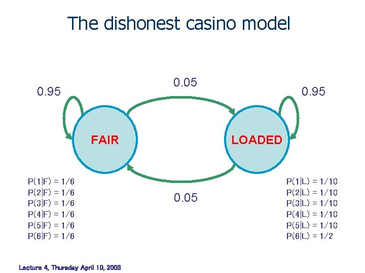
The dishonest casino model 0. 05 0. 95 FAIR P(1|F) P(2|F) P(3|F) P(4|F) P(5|F) P(6|F) = = = 1/6 1/6 1/6 Lecture 4, Thursday April 10, 2003 0. 95 LOADED 0. 05 P(1|L) P(2|L) P(3|L) P(4|L) P(5|L) P(6|L) = = = 1/10 1/10 1/2

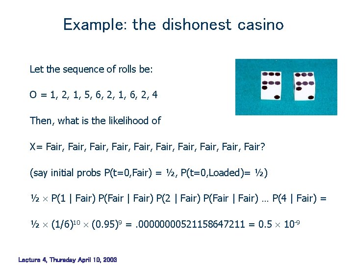
Example: the dishonest casino Let the sequence of rolls be: O = 1, 2, 1, 5, 6, 2, 1, 6, 2, 4 Then, what is the likelihood of X= Fair, Fair, Fair, Fair? (say initial probs P(t=0, Fair) = ½, P(t=0, Loaded)= ½) ½ P(1 | Fair) P(Fair | Fair) P(2 | Fair) P(Fair | Fair) … P(4 | Fair) = ½ (1/6)10 (0. 95)9 =. 0000521158647211 = 0. 5 10 -9 Lecture 4, Thursday April 10, 2003

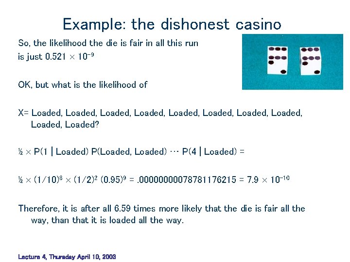
Example: the dishonest casino So, the likelihood the die is fair in all this run is just 0. 521 10 -9 OK, but what is the likelihood of X= Loaded, Loaded, Loaded, Loaded? ½ P(1 | Loaded) P(Loaded, Loaded) … P(4 | Loaded) = ½ (1/10)8 (1/2)2 (0. 95)9 =. 0000078781176215 = 7. 9 10 -10 Therefore, it is after all 6. 59 times more likely that the die is fair all the way, than that it is loaded all the way. Lecture 4, Thursday April 10, 2003

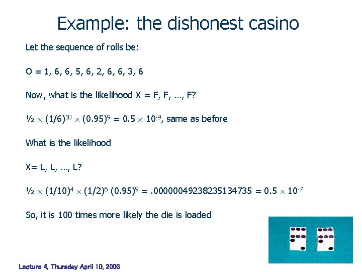
Example: the dishonest casino Let the sequence of rolls be: O = 1, 6, 6, 5, 6, 2, 6, 6, 3, 6 Now, what is the likelihood X = F, F, …, F? ½ (1/6)10 (0. 95)9 = 0. 5 10 -9, same as before What is the likelihood X= L, L, …, L? ½ (1/10)4 (1/2)6 (0. 95)9 =. 00000049238235134735 = 0. 5 10 -7 So, it is 100 times more likely the die is loaded Lecture 4, Thursday April 10, 2003

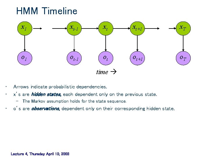
HMM Timeline x 1 xt-1 xt xt+1 x. T o 1 ot-1 ot ot+1 o. T time • • Arrows indicate probabilistic dependencies. x’s are hidden states, each dependent only on the previous state. – The Markov assumption holds for the state sequence. • o’s are observations, dependent only on their corresponding hidden state. Lecture 4, Thursday April 10, 2003

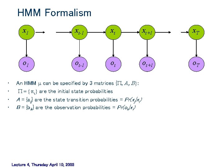
HMM Formalism • • x 1 xt-1 xt xt+1 x. T o 1 ot-1 ot ot+1 o. T An HMM can be specified by 3 matrices { , A, B}: = { i} are the initial state probabilities A = {aij} are the state transition probabilities = Pr(xj|xi) B = {bik} are the observation probabilities = Pr(ok|xi) Lecture 4, Thursday April 10, 2003

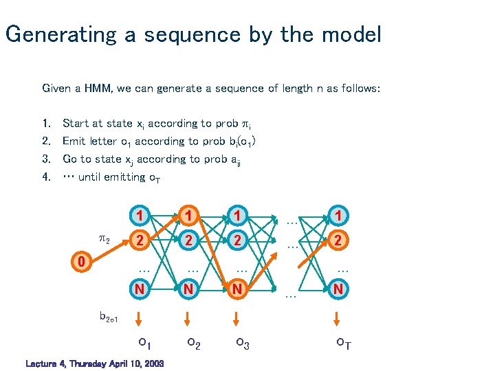
Generating a sequence by the model Given a HMM, we can generate a sequence of length n as follows: 1. 2. 3. 4. Start at state xi according to prob i Emit letter o 1 according to prob bi(o 1) Go to state xj according to prob aij … until emitting o. T 2 0 1 1 1 … 1 2 2 2 … … … N N N K o 1 o 2 o 3 … … N b 2 o 1 Lecture 4, Thursday April 10, 2003 o. T

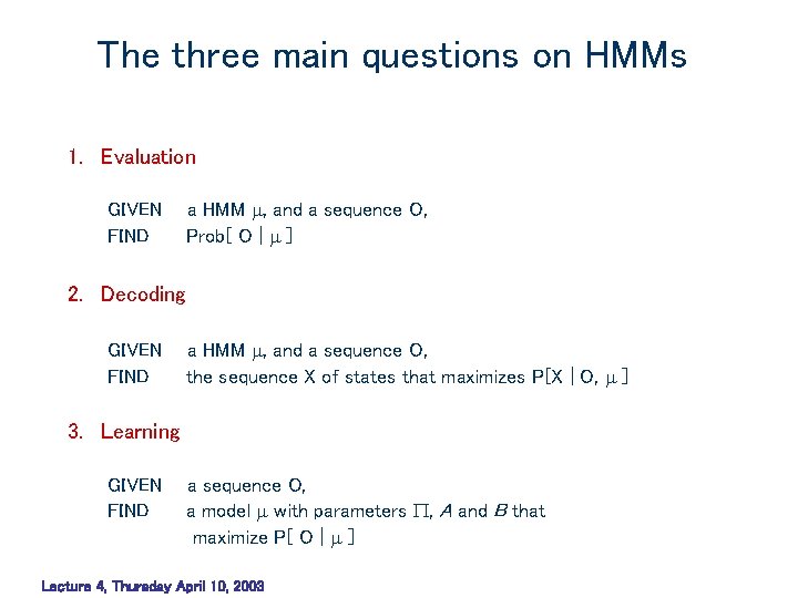
The three main questions on HMMs 1. Evaluation a HMM , and a sequence O, Prob[ O | ] GIVEN FIND 2. Decoding GIVEN FIND a HMM , and a sequence O, the sequence X of states that maximizes P[X | O, ] 3. Learning GIVEN FIND a sequence O, a model with parameters , A and B that maximize P[ O | ] Lecture 4, Thursday April 10, 2003

Problem 1: Evaluation Find the likelihood a sequence is generated by the model Lecture 4, Thursday April 10, 2003

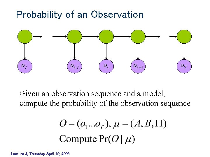
Probability of an Observation o 1 ot-1 ot ot+1 o. T Given an observation sequence and a model, compute the probability of the observation sequence Lecture 4, Thursday April 10, 2003

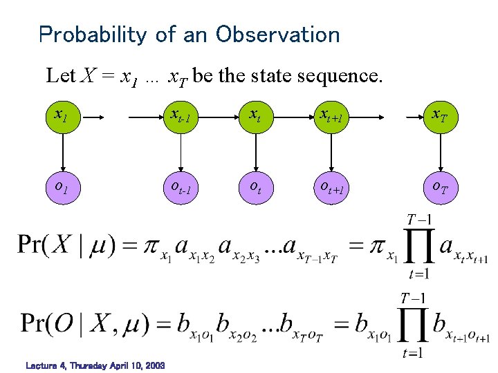
Probability of an Observation Let X = x 1 … x. T be the state sequence. x 1 xt-1 xt xt+1 x. T o 1 ot-1 ot ot+1 o. T Lecture 4, Thursday April 10, 2003

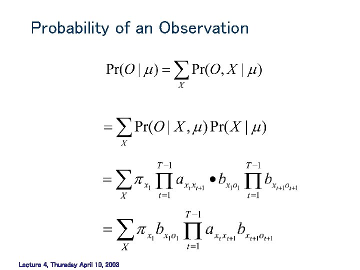
Probability of an Observation Lecture 4, Thursday April 10, 2003

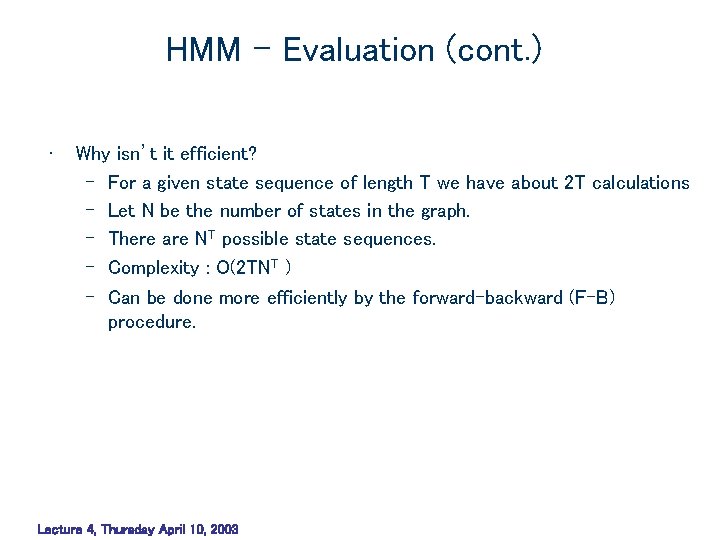
HMM – Evaluation (cont. ) • Why isn’t it efficient? – For a given state sequence of length T we have about 2 T calculations – Let N be the number of states in the graph. – There are NT possible state sequences. – Complexity : O(2 TNT ) – Can be done more efficiently by the forward-backward (F-B) procedure. Lecture 4, Thursday April 10, 2003

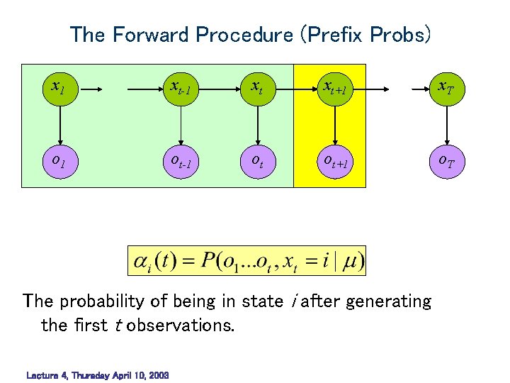
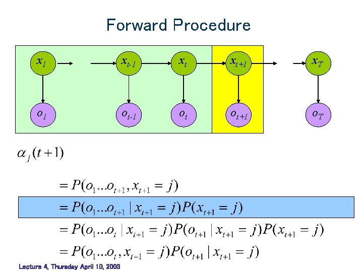
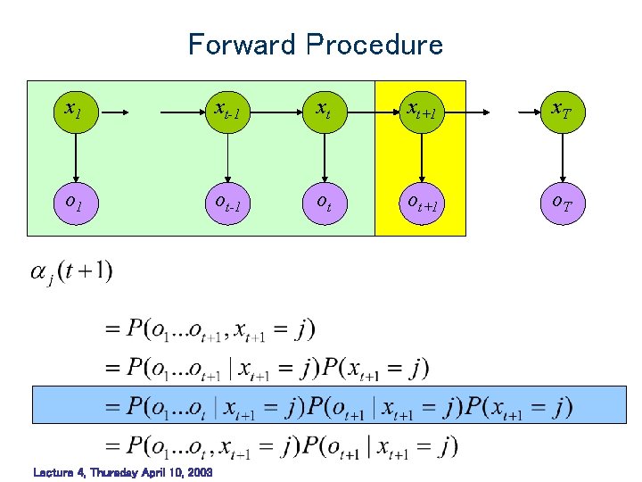
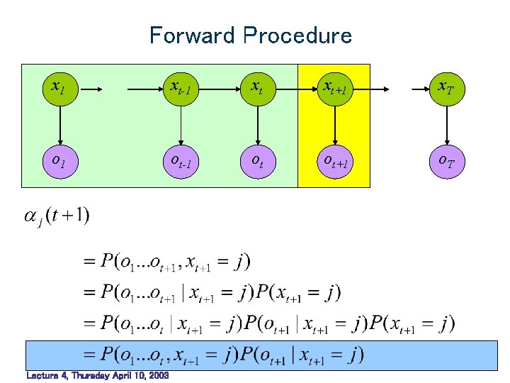
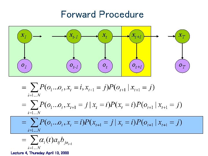
The Forward Procedure (Prefix Probs) x 1 xt-1 xt xt+1 x. T o 1 ot-1 ot ot+1 o. T The probability of being in state i after generating the first t observations. Lecture 4, Thursday April 10, 2003

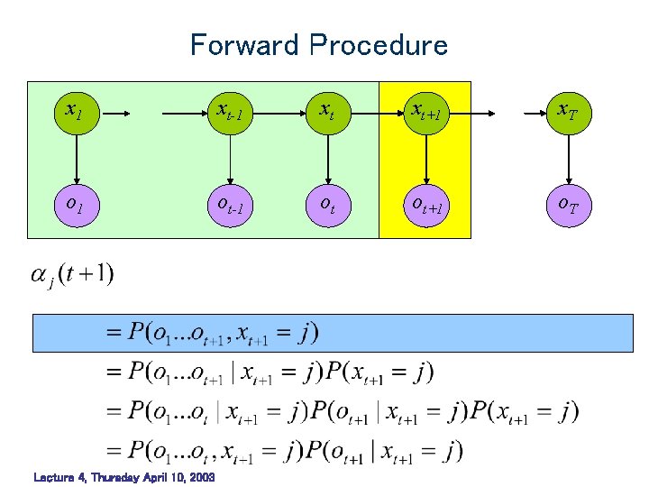
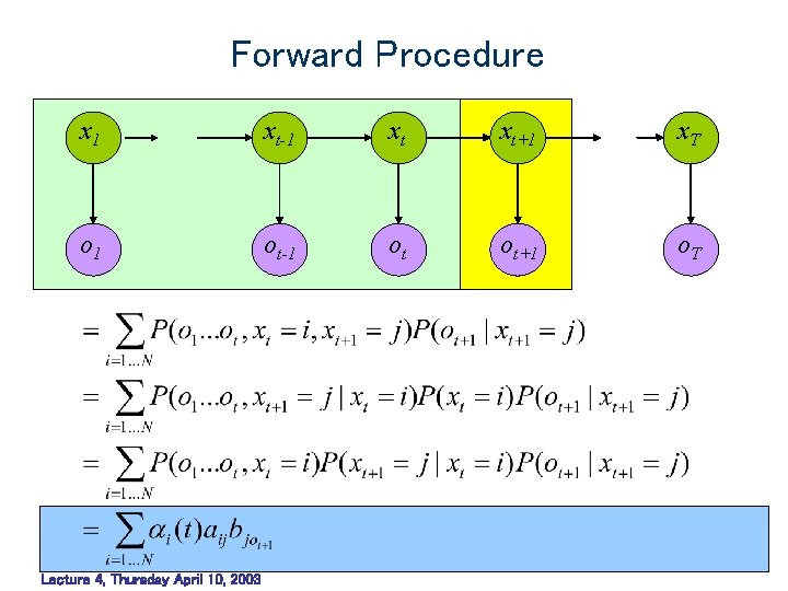
Forward Procedure x 1 xt-1 xt xt+1 x. T o 1 ot-1 ot ot+1 o. T Lecture 4, Thursday April 10, 2003

Forward Procedure x 1 xt-1 xt xt+1 x. T o 1 ot-1 ot ot+1 o. T Lecture 4, Thursday April 10, 2003

Forward Procedure x 1 xt-1 xt xt+1 x. T o 1 ot-1 ot ot+1 o. T Lecture 4, Thursday April 10, 2003

Forward Procedure x 1 xt-1 xt xt+1 x. T o 1 ot-1 ot ot+1 o. T Lecture 4, Thursday April 10, 2003

Forward Procedure x 1 xt-1 xt xt+1 x. T o 1 ot-1 ot ot+1 o. T Lecture 4, Thursday April 10, 2003

Forward Procedure x 1 xt-1 xt xt+1 x. T o 1 ot-1 ot ot+1 o. T Lecture 4, Thursday April 10, 2003

Forward Procedure x 1 xt-1 xt xt+1 x. T o 1 ot-1 ot ot+1 o. T Lecture 4, Thursday April 10, 2003

Forward Procedure x 1 xt-1 xt xt+1 x. T o 1 ot-1 ot ot+1 o. T Lecture 4, Thursday April 10, 2003

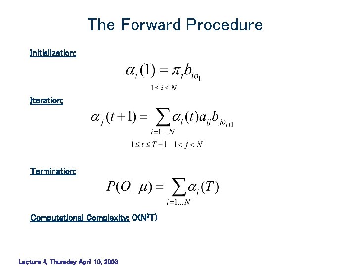
The Forward Procedure Initialization: Iteration: Termination: Computational Complexity: O(N 2 T) Lecture 4, Thursday April 10, 2003

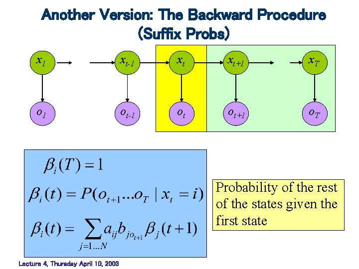
Another Version: The Backward Procedure (Suffix Probs) x 1 xt-1 xt xt+1 x. T o 1 ot-1 ot ot+1 o. T Probability of the rest of the states given the first state Lecture 4, Thursday April 10, 2003

Problem 2: Decoding Find the best state sequence Lecture 4, Thursday April 10, 2003

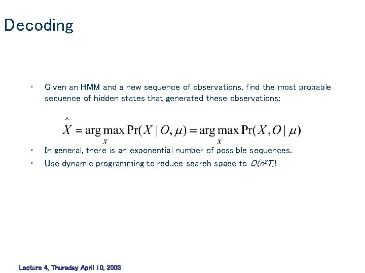
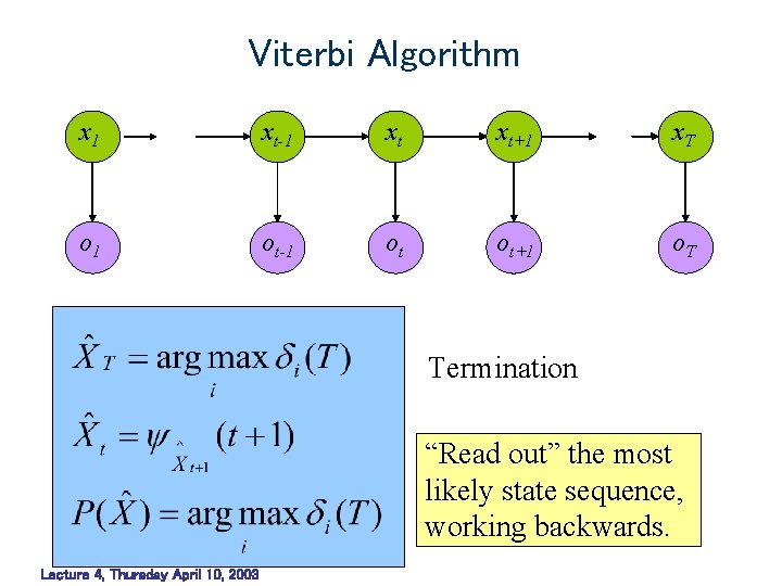
Decoding • Given an HMM and a new sequence of observations, find the most probable sequence of hidden states that generated these observations: • • In general, there is an exponential number of possible sequences. Use dynamic programming to reduce search space to O(n 2 T). Lecture 4, Thursday April 10, 2003

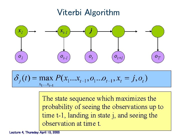
Viterbi Algorithm x 1 xt-1 j o 1 ot-1 ot ot+1 o. T The state sequence which maximizes the probability of seeing the observations up to time t-1, landing in state j, and seeing the observation at time t. Lecture 4, Thursday April 10, 2003

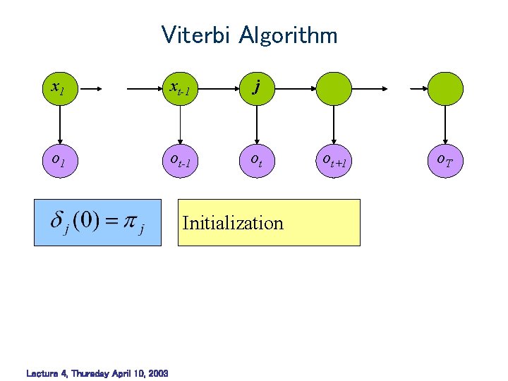
Viterbi Algorithm x 1 xt-1 j o 1 ot-1 ot Initialization Lecture 4, Thursday April 10, 2003 ot+1 o. T

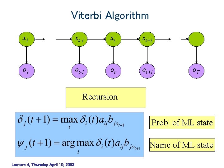
Viterbi Algorithm x 1 xt-1 xt xt+1 o 1 ot-1 ot ot+1 o. T Recursion Prob. of ML state Name of ML state Lecture 4, Thursday April 10, 2003

Viterbi Algorithm x 1 xt-1 xt xt+1 x. T o 1 ot-1 ot ot+1 o. T Termination “Read out” the most likely state sequence, working backwards. Lecture 4, Thursday April 10, 2003

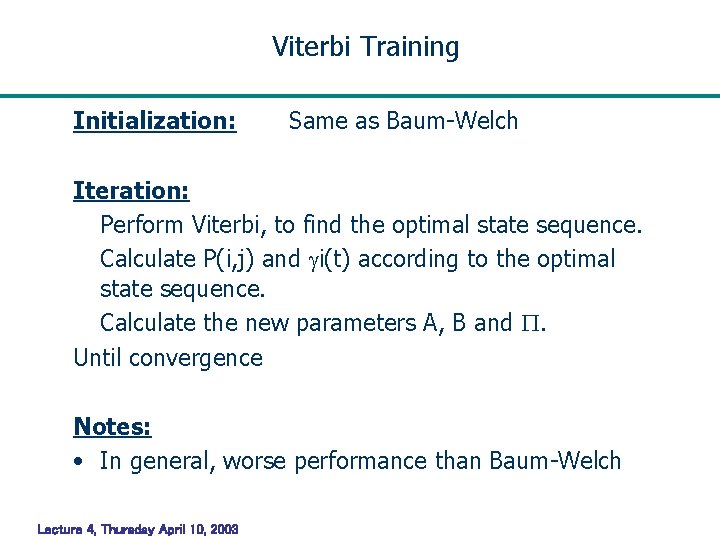
Viterbi Training Initialization: Same as Baum-Welch Iteration: Perform Viterbi, to find the optimal state sequence. Calculate P(i, j) and i(t) according to the optimal state sequence. Calculate the new parameters A, B and . Until convergence Notes: • In general, worse performance than Baum-Welch Lecture 4, Thursday April 10, 2003

Problem 3: Learning Re-estimate the parameters of the model based on training data Lecture 4, Thursday April 10, 2003

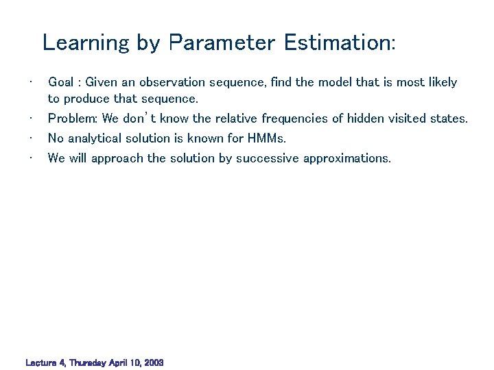
Learning by Parameter Estimation: • • Goal : Given an observation sequence, find the model that is most likely to produce that sequence. Problem: We don’t know the relative frequencies of hidden visited states. No analytical solution is known for HMMs. We will approach the solution by successive approximations. Lecture 4, Thursday April 10, 2003

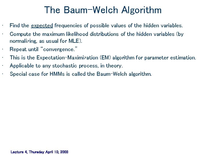
The Baum-Welch Algorithm • • • Find the expected frequencies of possible values of the hidden variables. Compute the maximum likelihood distributions of the hidden variables (by normalizing, as usual for MLE). Repeat until “convergence. ” This is the Expectation-Maximization (EM) algorithm for parameter estimation. Applicable to any stochastic process, in theory. Special case for HMMs is called the Baum-Welch algorithm. Lecture 4, Thursday April 10, 2003

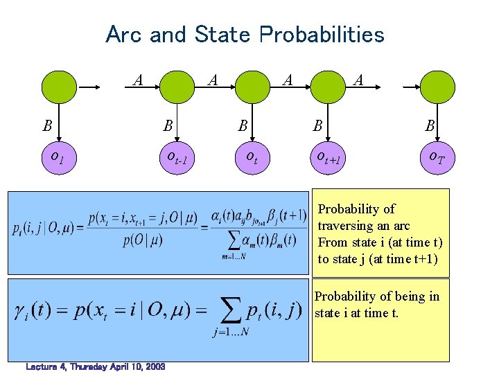
Arc and State Probabilities A B o 1 ot-1 A B ot A B B ot+1 o. T Probability of traversing an arc From state i (at time t) to state j (at time t+1) Probability of being in state i at time t. Lecture 4, Thursday April 10, 2003

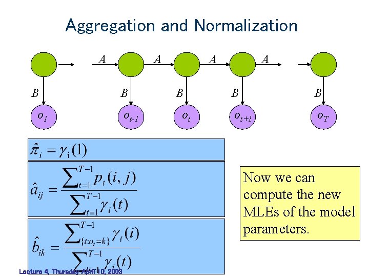
Aggregation and Normalization A B o 1 ot-1 A B ot A B B ot+1 o. T Now we can compute the new MLEs of the model parameters. Lecture 4, Thursday April 10, 2003

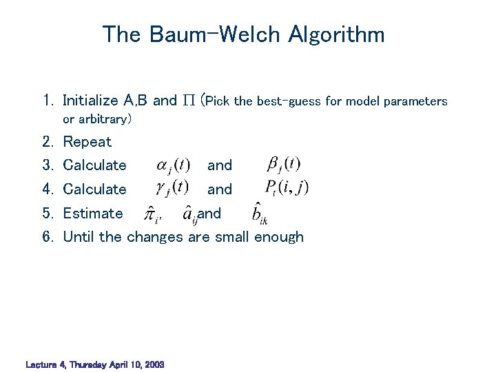
The Baum-Welch Algorithm 1. Initialize A, B and (Pick the best-guess for model parameters or arbitrary) 2. 3. 4. 5. 6. Repeat Calculate and Estimate , and Until the changes are small enough Lecture 4, Thursday April 10, 2003

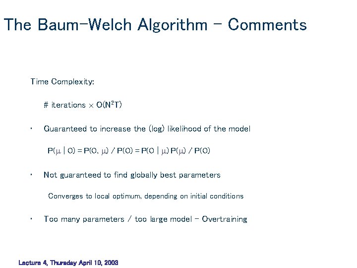
The Baum-Welch Algorithm – Comments Time Complexity: # iterations O(N 2 T) • Guaranteed to increase the (log) likelihood of the model P( | O) = P(O, ) / P(O) = P(O | ) P( ) / P(O) • Not guaranteed to find globally best parameters Converges to local optimum, depending on initial conditions • Too many parameters / too large model - Overtraining Lecture 4, Thursday April 10, 2003

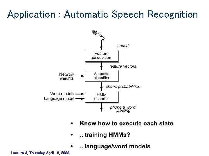
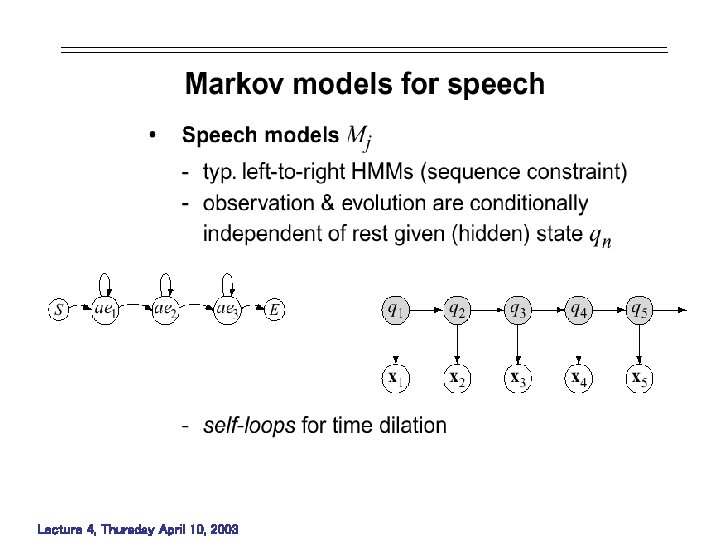
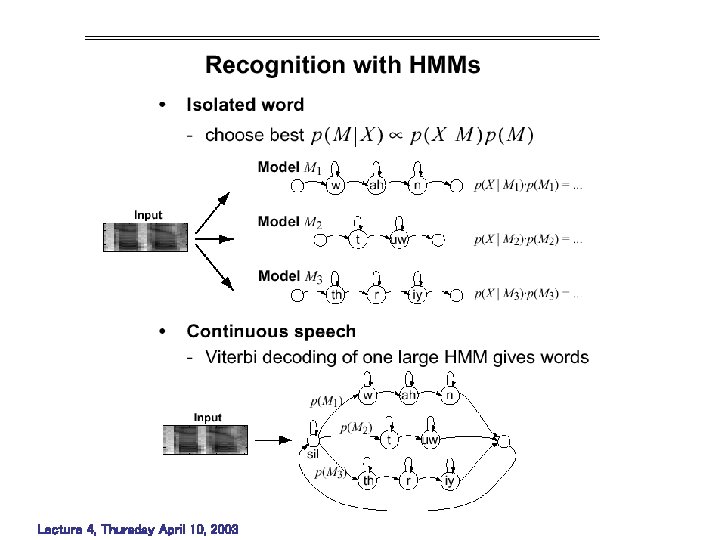
Application : Automatic Speech Recognition Lecture 4, Thursday April 10, 2003

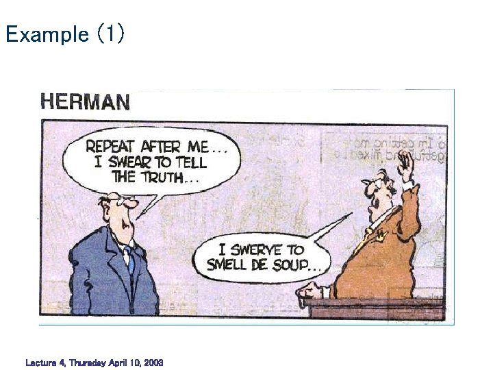
Example (1) Lecture 4, Thursday April 10, 2003

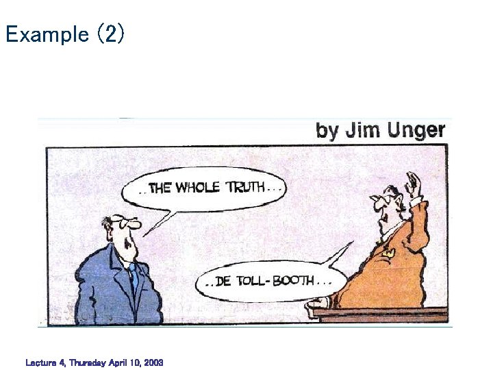
Example (2) Lecture 4, Thursday April 10, 2003

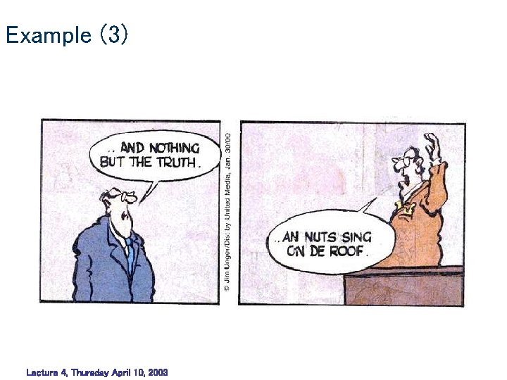
Example (3) Lecture 4, Thursday April 10, 2003

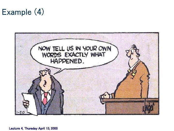
Example (4) Lecture 4, Thursday April 10, 2003

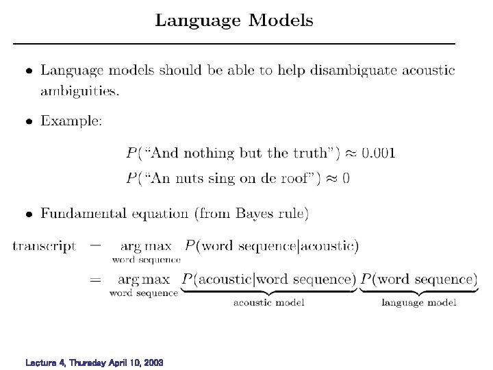
Lecture 4, Thursday April 10, 2003

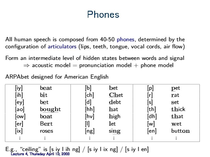
Phones Lecture 4, Thursday April 10, 2003

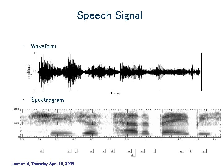
Speech Signal • Waveform • Spectrogram Lecture 4, Thursday April 10, 2003

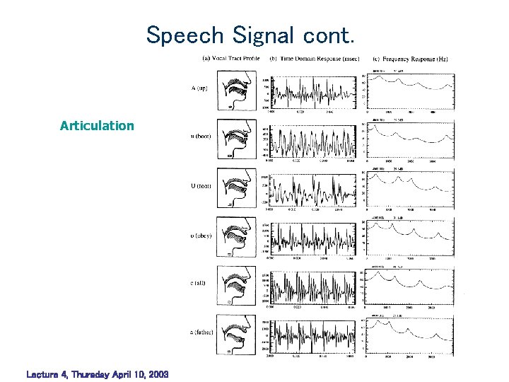
Speech Signal cont. Articulation Lecture 4, Thursday April 10, 2003

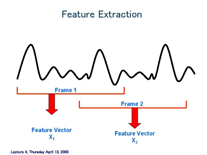
Feature Extraction Frame 1 Frame 2 Feature Vector X 1 Lecture 4, Thursday April 10, 2003 Feature Vector X 2

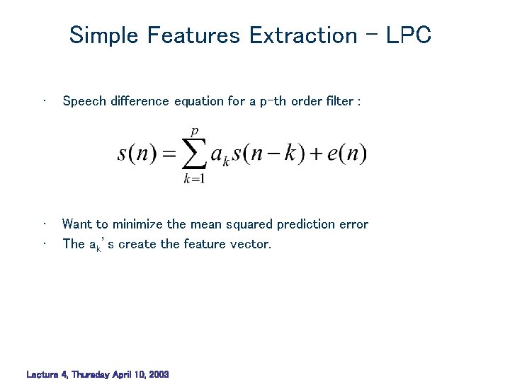
Simple Features Extraction - LPC • Speech difference equation for a p-th order filter : • • Want to minimize the mean squared prediction error The ak’s create the feature vector. Lecture 4, Thursday April 10, 2003

Lecture 4, Thursday April 10, 2003

Lecture 4, Thursday April 10, 2003