Heuristics CPSC 386 Artificial Intelligence Ellen Walker Hiram

Heuristics CPSC 386 Artificial Intelligence Ellen Walker Hiram College

Informed Search Strategies • Also called heuristic search • All are variations of best-first search – The next node to expand is the one “most likely” to lead to a solution – Priority queue, like uniform cost search, but priority is based on additional knowledge of the problem – The priority function for the priority queue is usually called f(n)

Heuristic Function • Heuristic, from Greek for “good” • Heuristic function, h(n) = estimated cost from the current state to the goal • Therefore, our best estimate of total path cost is g(n) + h(n) – Recall, g(n) is cost from initial state to current state

In A*, better h means better search • When h = cost to the goal, – Only nodes on correct path are expanded – Optimal solution is found • When h < cost to the goal, – Additional nodes are expanded – Optimal solution is found • When h > cost to the goal – Optimal solution can be overlooked

Pruning the Search Tree • In A* search, if h is too big, it will prevent the node (and its successors, grand-successors, etc. ) from ever being expanded • This is called “pruning” (like removing branches from a tree) • Pruning the tree reduces the search below exponential – Only if a good heuristic is available

Costs of A* • Time – The better the heuristic, the less time • Best case: h is perfect, O(d) • Worst admissible case: h is 0, O(bd), i. e. bfs • Space – All nodes (open and closed list) are saved in case of repetition – This is exponential (bd or worse). – A* generally runs out of space before it runs out of time

Memory-bounded Heuristic Search • Iterative Deepening A* (IDA*) – Like iterative deepening, but cutoff at (g+h)>max, rather than depth >max – At each iteration, cutoff is first f-cost that exceeds the cost of the node at the previous iteration. • Recursive BFS (see textbook, fig 4. 5) • Simple Memory Bounded A* (SMA*) – Set max memory bound – If memory is “full”, to add a node drop the worst (g+h) node that’s already stored – Expands newest best leaf, deletes oldest worst leaf

Backed-up Values • The (real) f-value of any node in a path is the same as the f-value of the solution • Therefore, you can update f of parent to best f of a child. (This also helps when revisiting a node from a different parent) • If you have to “forget” deeper nodes, their consequences are remembered in the parent • (This concept is used more prominently in adversary games)

Comparing Heuristic Functions • An admissible heuristic function never overestimates the distance to the goal. • The function h=0 is the least useful admissible function. • Given 2 admissible heuristic functions (h 1 and h 2), h 1 dominates h 2 if h 1(n)≥ h 2(n) for any node n • The perfect h function is dominant over all other admissible heuristic functions • Dominant admissible heuristic functions are better

Combining Heuristic Functions • Every admissible heuristic is <= the actual distance to goal • Therefore, if you have 2 admissible heuristics, the higher value is closer to the goal. • If you have 2 or more heuristics, you can therefore combine them into a better one by taking the maximum value for any state. • Useful when you have a set of heuristics where no one is dominant

Finding Heuristic Functions: Relaxed Problems • Remove constraints from the original problem to generate a “relaxed problem” • Cost of optimal solution to relaxed problem is admissable heuristic for original problem – Because a solution to the original problem also solves the relaxed problem (at a cost ≥ relaxed solution cost)

8 -puzzle examples • Number of tiles out of place – Relax constraint that tiles must move into empty squares, and that tiles must move into adjacent squares • Manhattan distance to solution – Relax (only) constraint that tiles must move into empty squares

Finding Heuristic Functions: Subproblems • Consider solving only part of the problem – Example: getting 1, 2, 3 and 4 of 8 -puzzle into place • Again, exact solutions to subproblems are admissable heuristics • Store subproblem solutions in a pattern database, look up heuristic – – # patterns is much smaller than state space! Generate database by working backwards from the solution If multiple subproblems apply, take the max If multiple disjoint subproblems apply, heuristics can be added

Finding Heuristic Functions: Learning • Take experience and learn a function • Each “experience” is a start state and the actual cost of the solution • Learn from “features” of a state that are relevant to a solution, rather than the state itself (helps generalization) – Generate “many” states with a given feature and determine average distance – Combine information from multiple features • h(n) = c 1 * x 1(n) + c 2 * x 2(n)… where x 1, x 2 are features

Local Search Algorithms • Instead of considering the whole state space, consider only the current state • Limits necessary memory; paths not retained • Amenable to large or continuous (infinite) state spaces where exhaustive algorithms aren’t possible • Local search algorithms can’t backtrack!

Optimization • Given measure of goodness (of fit) • Find optimal parameters (e. g correspondences) • That maximize goodness measure (or minimize badness measure) • Optimization techniques – – Direct (closed-form) Search (generate-test) Heuristic search (e. g Hill Climbing) Genetic Algorithm

Direct Optimization • The slope of a function at the maximum or minimum is 0 – Function is neither growing nor shrinking – True at global, but also local extreme points • Find where the slope is zero and you find extrema! • (If you have the equation, use calculus (first derivative=0) but watch out for “shoulders”

Hill Climbing • Consider all possible successors as “one step” from the current state on the landscape. • At each iteration, go to – The best successor (steepest ascent) – Any uphill move (first choice) – Any uphill move but steeper is more probable (stochastic) • All variations get stuck at local maxima

Issues in Hill Climbing • Local maxima = no uphill step – Algorithms on previous slide fail (not complete) – Allow “random restart” which is complete, but might take a very long time • Plateau = all steps equal (flat or shoulder) – Must move to equal state to make progress, but no indication of the correct direction • Ridge = narrow path of maxima, but might have to go down to go up (e. g. diagonal ridge in 4 -direction space)

Simulated Annealing • Figure 4. 14, simulate gradual cooling to low-energy crystalline state • Algorithm is randomized: take a step if random number is less than a value based on both the objective function and the Temperature. • When Temperature is high, chance of going toward a higher value of optimization function J(x) is greater. • Note higher dimension: “perturb parameter vector” vs. “look at next and previous value”.

Local Beam Search • Keep track of K local searches at once • At each step, generate all successors and keep the best K • (Localized version of memory-bounded A*) • Stochastic: choose K states at random, but probability of state being chosen is proportional to its goodness

Genetic Algorithm • Quicker but randomized searching for an optimal parameter vector • Operations – Crossover (2 parents -> 2 children) – Mutation (one “bit”) • Basic structure – Create population – Perform crossover & mutation (on fittest) – Keep only fittest children

Example: “Hello, World” • Initial population is 2048 random strings of length 12 • Fitness of an individual is calculated by comparing each letter to its corresponding letter in the target phrase and adding up the differences • Top 10% of population is retained, remaining 90% is created by crossover of top 50% of population with 25% chance of mutation – Crossover: choose a random position and swap substrings – Mutation: choose a random position and replace by a random character Source: http: //generation 5. org/content/2003/gahelloworld. asp

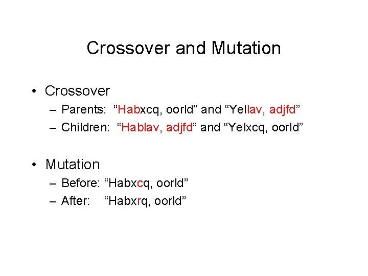
Crossover and Mutation • Crossover – Parents: “Habxcq, oorld” and “Yellav, adjfd” – Children: “Hablav, adjfd” and “Yelxcq, oorld” • Mutation – Before: “Habxcq, oorld” – After: “Habxrq, oorld”

Genetic Algorithm: Why does it work? • Children carry parts of their parents’ data • Only “good” parents can reproduce – Children are at least as “good” as parents? • No, but “worse” children don’t last long • Large population allows many “current points” in search – Can consider several regions (watersheds) at once

Genetic Algorithm: Issues & Pitfalls • Representation – Children (after crossover) should be similar to parent, not random – Binary representation of numbers isn’t good - what happens when you crossover in the middle of a number? – Need “reasonable” breakpoints for crossover (e. g. between R, xcenter and ycenter but not within them) • “Cover” – Population should be large enough to “cover” the range of possibilities – Information shouldn’t be lost too soon – Mutation helps with this issue

Experimenting With Genetic Algorithms • Be sure you have a reasonable “goodness” criterion • Choose a good representation (including methods for crossover and mutation) • Generate a sufficiently random, large enough population • Run the algorithm “long enough” • Find the “winners” among the population • Variations: multiple populations, keeping vs. not keeping parents, “immigration / emigration”, mutation rate, etc.

Summary: Search Techniques • Exhaustive – Depth-first, Breadth First – Uniform cost – Iterative Deepening • Best-first (heuristic) – Greedy – A* – Memory-bounded (beam, mb. A*) • Local heuristic – Hill-climbing (steepest, any upward, random restart) – Simulated annealing (stochastic) – Genetic Algorithm (highly parallel, stochastic)