Help Statistics Multiple testing Problems and some solutions

Help! Statistics! Multiple testing. Problems and some solutions. Hans Burgerhof j. g. m. burgerhof@umcg. nl February 12 2019

Help! Statistics! Lunchtime Lectures What? When? frequently used statistical methods and questions in a manageable timeframe for all researchers at the UMCG No knowledge of advanced statistics is required. do not Lectures take place every 2 nd Tuesday of the month, 12. 00 -13. 00 hrs. Who? Unit for Medical Statistics and Decision Making When? Where? What? Who? Feb 12 2019 Room 16 H. Burgerhof April 9 2019 Room 16 June 11 2019 ? Multiple testing. Problems and some solutions Kaplan-Meier survival curves and the log rank test ? D. Postmus ? Slides can be downloaded from http: //www. rug. nl/research/epidemiology/download-area 2

Program Today 1. Multiple testing. What is the problem? 2. (Stochastically) independent tests versus dependent tests 3. Controlling the Familywise Error Rate (FWER) 4. Controlling the False Discovery Rate (FDR) 5. Some references (for finding more solutions)

Type I and Type II errors for a statistical test H 0: effect new treatment = effect standard treatment H 1: effect new treatment > effect standard treatment Decision Reality H 0 true H 0 not true H 0 true OK Probability: 1 - α Type I error Probability: α H 0 not true Type II error Probability: β OK power Probability: 1 - The significance level is generally 0. 05; We allow 5% probability to reject H 0, while in fact it is true

The classical problem of multiple testing • In statistical testing, we usually define the significance level α at 0. 05. This means we accept a probability of 0. 05 to reject a null hypothesis, while in fact the null hypothesis is true • This is called the Comparison-wise error rate (CWER) • What can we say about the probability of rejecting at least one null hypothesis if we have more than one hypothesis to test? Chance capitalisation! “Overall alpha” Family-wise error rate (FWER)

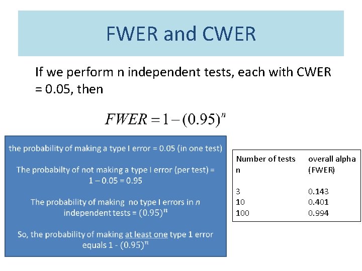
FWER and CWER If we perform n independent tests, each with CWER = 0. 05, then Number of tests n overall alpha (FWER) 3 10 100 0. 143 0. 401 0. 994

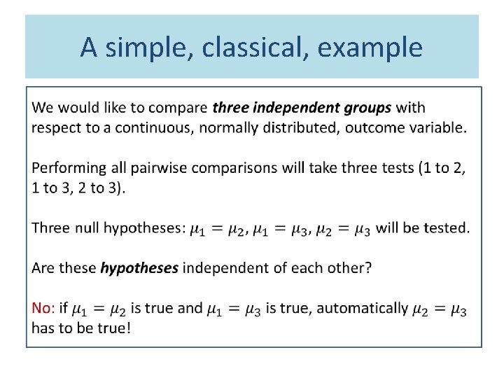
A simple, classical, example

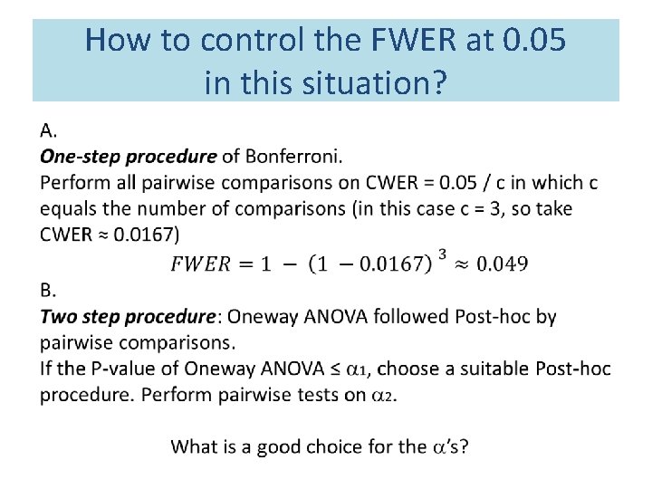
How to control the FWER at 0. 05 in this situation?

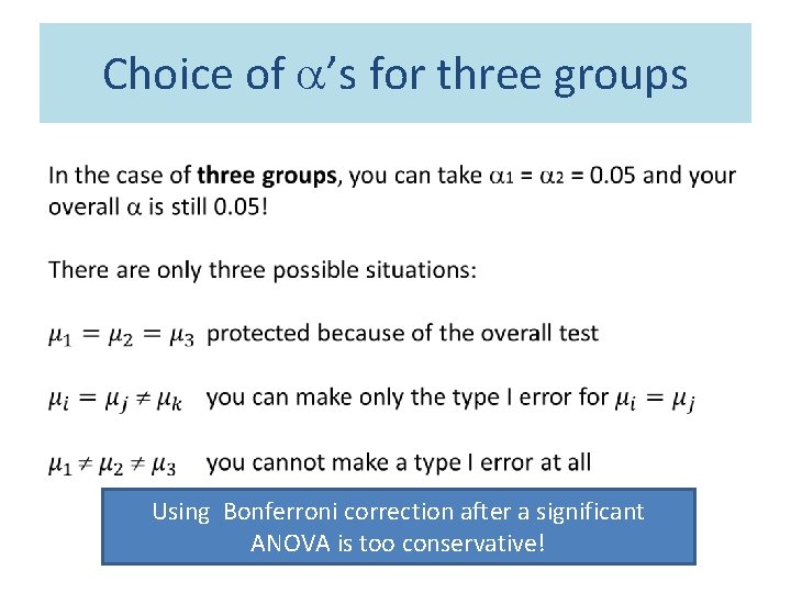
Choice of ’s for three groups Using Bonferroni correction after a significant ANOVA is too conservative!

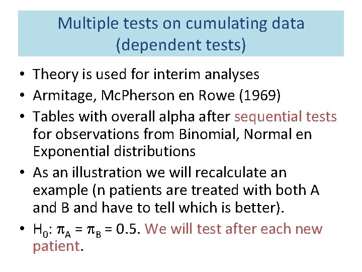
Multiple tests on cumulating data (dependent tests) • Theory is used for interim analyses • Armitage, Mc. Pherson en Rowe (1969) • Tables with overall alpha after sequential tests for observations from Binomial, Normal en Exponential distributions • As an illustration we will recalculate an example (n patients are treated with both A and B and have to tell which is better). • H 0: A = B = 0. 5. We will test after each new patient.

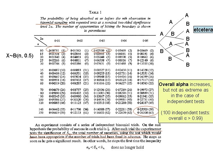
A A A B X~B(n, 0. 5) B B A etcetera B A B Overall alpha increases, but not as extreme as in the case of independent tests (100 independent tests: overall α > 0. 99) does no longer hold

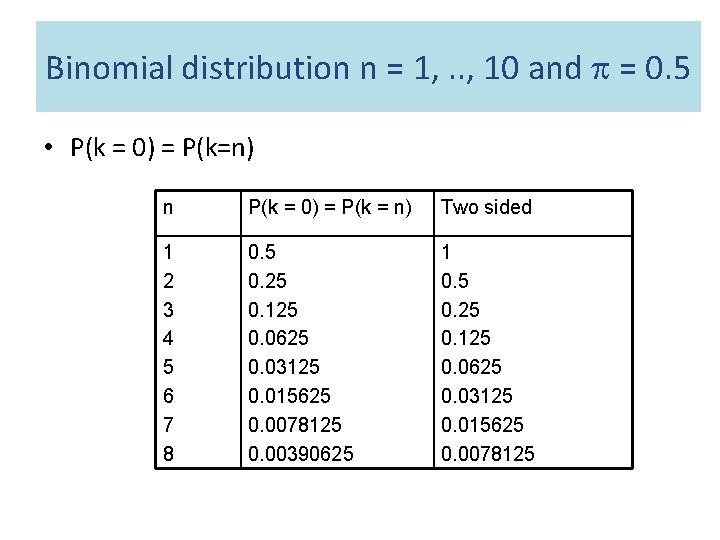
Binomial distribution n = 1, . . , 10 and = 0. 5 • P(k = 0) = P(k=n) n P(k = 0) = P(k = n) Two sided 1 2 3 4 5 6 7 8 0. 5 0. 25 0. 125 0. 0625 0. 03125 0. 015625 0. 0078125 0. 00390625 1 0. 5 0. 25 0. 125 0. 0625 0. 03125 0. 015625 0. 0078125

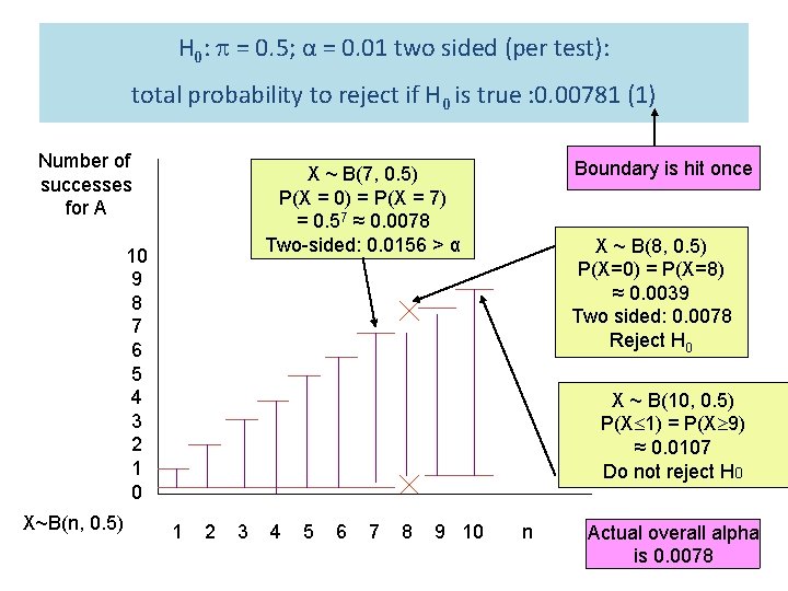
H 0: = 0. 5; α = 0. 01 two sided (per test): total probability to reject if H 0 is true : 0. 00781 (1) Number of successes for A 10 9 8 7 6 5 4 3 2 1 0 X~B(n, 0. 5) Boundary is hit once X ~ B(7, 0. 5) P(X = 0) = P(X = 7) = 0. 57 ≈ 0. 0078 Two-sided: 0. 0156 > α X ~ B(8, 0. 5) P(X=0) = P(X=8) ≈ 0. 0039 Two sided: 0. 0078 Reject H 0 X ~ B(10, 0. 5) P(X 1) = P(X 9) ≈ 0. 0107 Do not reject H 0 1 2 3 4 5 6 7 8 9 10 n Actual overall alpha is 0. 0078

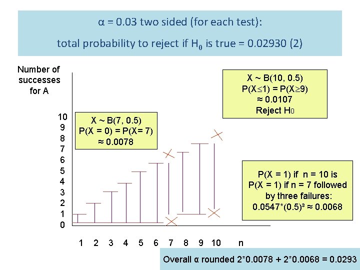
α = 0. 03 two sided (for each test): total probability to reject if H 0 is true = 0. 02930 (2) Number of successes for A 10 9 8 7 6 5 4 3 2 1 0 X ~ B(10, 0. 5) P(X 1) = P(X 9) ≈ 0. 0107 Reject H 0 X ~ B(7, 0. 5) P(X = 0) = P(X= 7) ≈ 0. 0078 P(X = 1) if n = 10 is P(X = 1) if n = 7 followed by three failures: 0. 0547*(0. 5)³ ≈ 0. 0068 1 2 3 4 5 6 7 8 9 10 n Overall α rounded 2*0. 0078 + 2*0. 0068 = 0. 0293

Many independent tests We are interested in genes, possibly related to a certain disease. Example: We have 100 candidate genes and compare their expressions in a group of diseased respondents with the expressions in a group of non-diseased respondents. We test 100 (more or less) independent tests (H 0: no effect). How to correct for multiple testing?

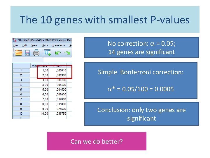
The 10 genes with smallest P-values No correction: = 0. 05; 14 genes are significant Simple Bonferroni correction: * = 0. 05/100 = 0. 0005 Conclusion: only two genes are significant Can we do better?

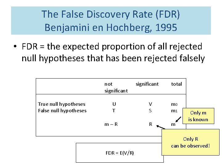
The False Discovery Rate (FDR) Benjamini en Hochberg, 1995 • FDR = the expected proportion of all rejected null hypotheses that has been rejected falsely not significant True null hypotheses False null hypotheses significant total U T V S m 0 m 1 m–R R m Only m is known Only R can be observed! FDR = E(V/R)

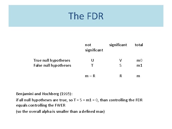
The FDR not significant True null hypotheses False null hypotheses significant total U T V S m 0 m 1 m–R R m Benjamini and Hochberg (1995): if all null hypotheses are true, so T = S = m 1 = 0, than controlling the FDR equals controlling the FWER (so the overall alpha is smaller than a defined max)

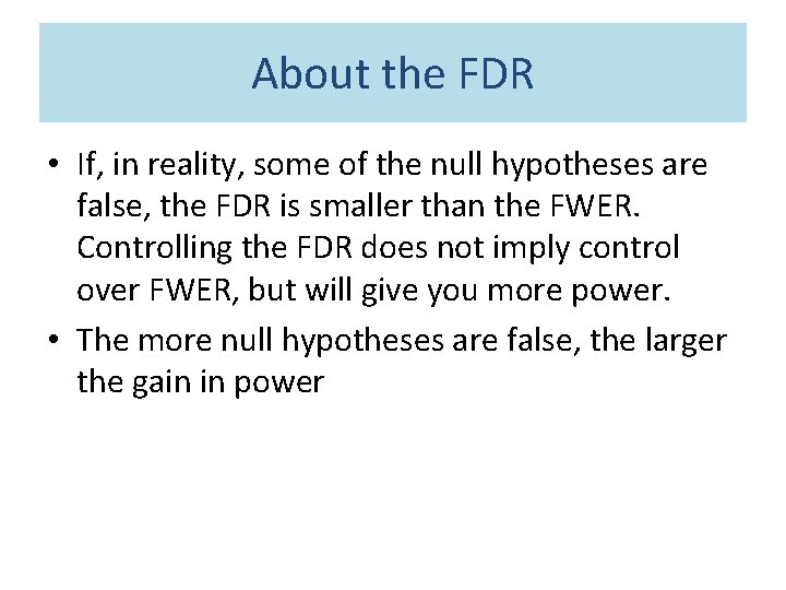
About the FDR • If, in reality, some of the null hypotheses are false, the FDR is smaller than the FWER. Controlling the FDR does not imply control over FWER, but will give you more power. • The more null hypotheses are false, the larger the gain in power

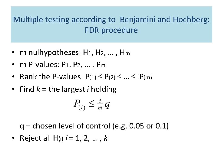
Multiple testing according to Benjamini and Hochberg: FDR procedure • • m nulhypotheses: H 1, H 2, … , Hm m P-values: P 1, P 2, … , Pm Rank the P-values: P(1) ≤ P(2) ≤ … ≤ P(m) Find k = the largest i holding q = chosen level of control (e. g. 0. 05 or 0. 1) • Reject all H(i) i = 1, 2, … , k

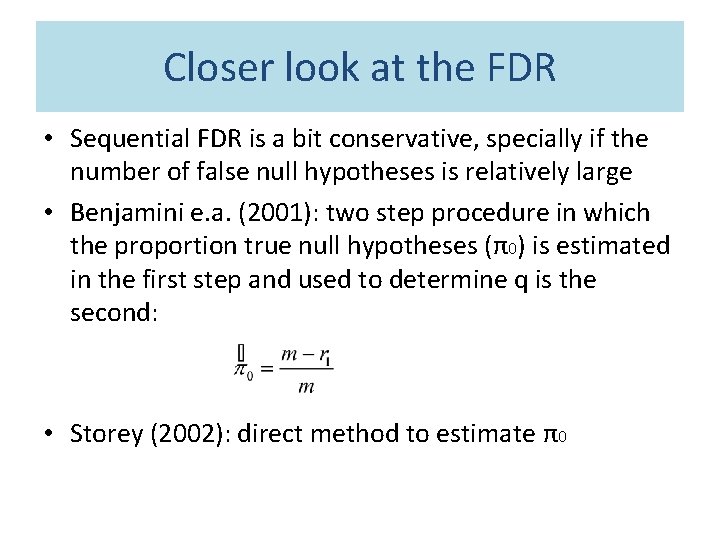
Closer look at the FDR • Sequential FDR is a bit conservative, specially if the number of false null hypotheses is relatively large • Benjamini e. a. (2001): two step procedure in which the proportion true null hypotheses (π0) is estimated in the first step and used to determine q is the second: • Storey (2002): direct method to estimate π0

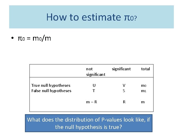
How to estimate π0? • π0 = m 0/m not significant True null hypotheses False null hypotheses significant total U T V S m 0 m 1 m–R R m What does the distribution of P-values look like, if the null hypothesis is true?

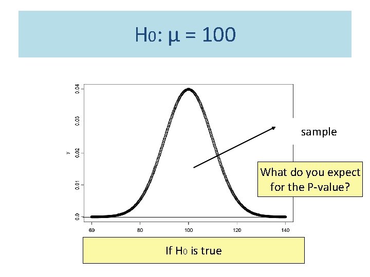
H 0: µ = 100 sample What do you expect for the P-value? If H 0 is true

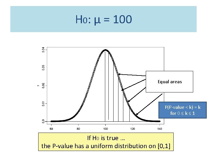
H 0: µ = 100 Equal areas P(P-value < k) = k for 0 ≤ k ≤ 1 If H 0 is true … the P-value has a uniform distribution on [0, 1]

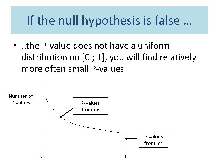
If the null hypothesis is false … • . . the P-value does not have a uniform distribution on [0 ; 1], you will find relatively more often small P-values Number of P-values from m 1 P-values from m 0 0 1

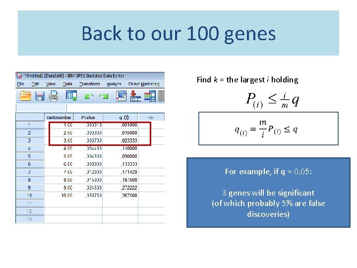
Back to our 100 genes Find k = the largest i holding (i) For example, if q = 0. 05: 3 genes will be significant (of which probably 5% are false discoveries)

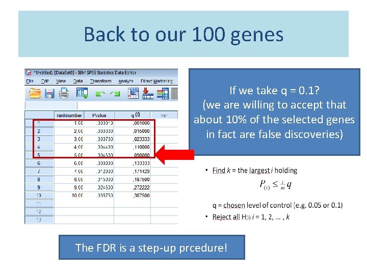
Back to our 100 genes (i) If we take q = 0. 1? (we are willing to accept that about 10% of the selected genes in fact are false discoveries) The FDR is a step-up prcedure!

literature • Armitage P. , Mc. Pherson K. and Rowe B. (1969) Journal of the Royal Statistical Society Series A. 132(2) 235 - 244 • Austin S. , Dialsingh I. and Altman N. (2014) Multiple hypothesis testing: a review. http: //personal. psu. edu/nsa 1/paper. Pdfs/Mult_Hyp_Review_final. pdf • Benjamini Y. and Hochberg Y. (1995). Controlling the False Discovery Rate: a practical and powerful approach to multiple testing. Journal of the Royal Statistical Society Series B, 289 -300 • Benjamini, Y. and Yekutieli, D. (2001). The control of the false discovery rate in multiple testing under dependency. Annals of Statistics, 29, 11651188. • Storey J. D. (2002). A direct approach to false discovery rates. Journal of the Royal Statistical Society Series B, 479 – 498.