HEDGING NONLINEAR RISK LINEAR AND NONLINEAR HEDGING Linear

HEDGING NONLINEAR RISK

LINEAR AND NONLINEAR HEDGING Linear hedging forwards and futures values are linearly related to the underlying risk factors Because linear combinations of normal random variables are also normally distributed, linear hedging maintains normal distributions Nonlinear hedging Options Since options can be replicated by dynamic trading of the underlying instruments, this also provides insights into the risks of active trading strategies BAHATTIN BUYUKSAHIN, CELSO BRUNETTI 2

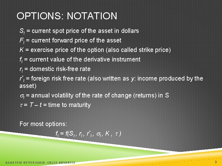
OPTIONS: NOTATION St = current spot price of the asset in dollars Ft = current forward price of the asset K = exercise price of the option (also called strike price) ft = current value of the derivative instrument rt = domestic risk-free rate r*t = foreign risk free rate (also written as y: income produced by the asset) t = annual volatility of the rate of change (returns) in S = T – t = time to maturity For most options: ft = f(St , r*t , K , ) BAHATTIN BUYUKSAHIN, CELSO BRUNETTI 3

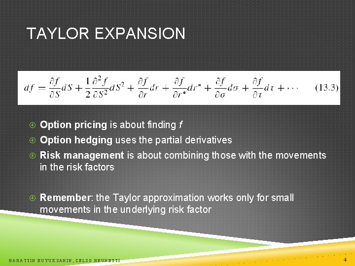
TAYLOR EXPANSION Option pricing is about finding f Option hedging uses the partial derivatives Risk management is about combining those with the movements in the risk factors Remember: the Taylor approximation works only for small movements in the underlying risk factor BAHATTIN BUYUKSAHIN, CELSO BRUNETTI 4

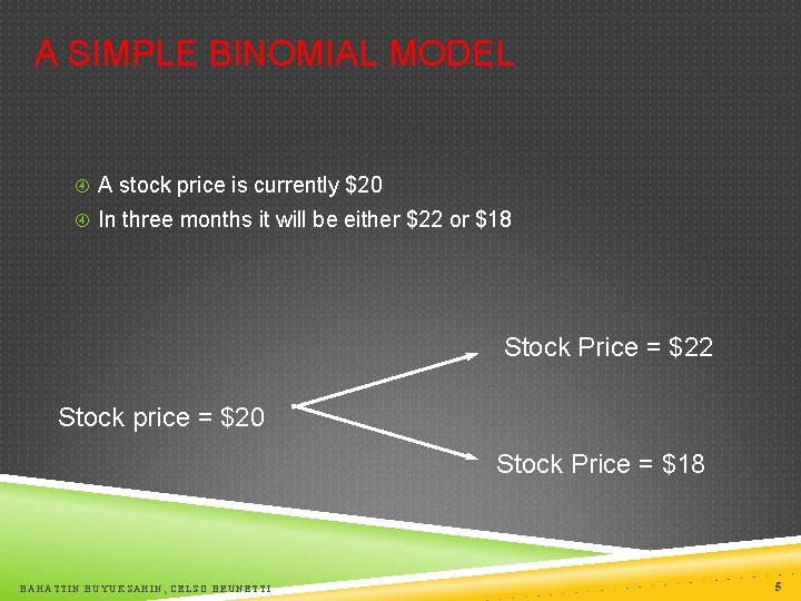
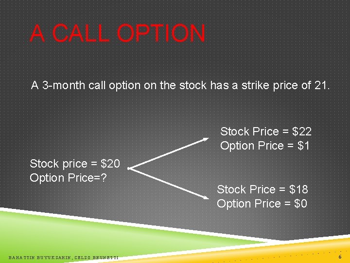
A SIMPLE BINOMIAL MODEL A stock price is currently $20 In three months it will be either $22 or $18 Stock Price = $22 Stock price = $20 Stock Price = $18 BAHATTIN BUYUKSAHIN, CELSO BRUNETTI 5

A CALL OPTION A 3 -month call option on the stock has a strike price of 21. Stock Price = $22 Option Price = $1 Stock price = $20 Option Price=? BAHATTIN BUYUKSAHIN, CELSO BRUNETTI Stock Price = $18 Option Price = $0 6

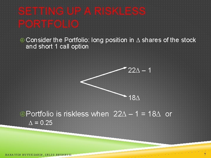
SETTING UP A RISKLESS PORTFOLIO Consider the Portfolio: long position in shares of the stock and short 1 call option 22 – 1 18 Portfolio is riskless when 22 – 1 = 18 or = 0. 25 BAHATTIN BUYUKSAHIN, CELSO BRUNETTI 7

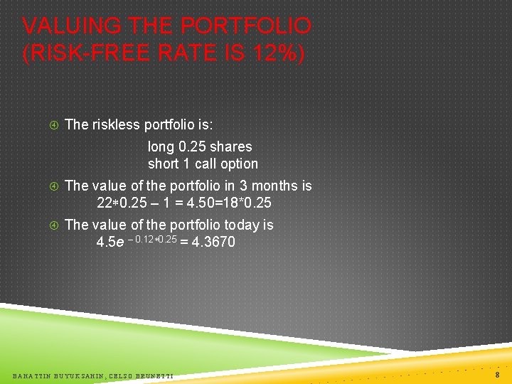
VALUING THE PORTFOLIO (RISK-FREE RATE IS 12%) The riskless portfolio is: long 0. 25 shares short 1 call option The value of the portfolio in 3 months is 22*0. 25 – 1 = 4. 50=18*0. 25 The value of the portfolio today is 4. 5 e – 0. 12*0. 25 = 4. 3670 BAHATTIN BUYUKSAHIN, CELSO BRUNETTI 8

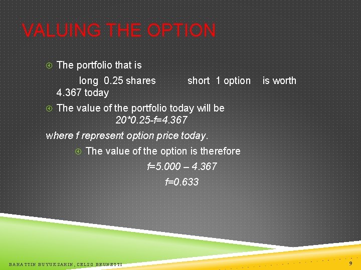
VALUING THE OPTION The portfolio that is long 0. 25 shares 4. 367 today short 1 option is worth The value of the portfolio today will be 20*0. 25 -f=4. 367 where f represent option price today. The value of the option is therefore f=5. 000 – 4. 367 f=0. 633 BAHATTIN BUYUKSAHIN, CELSO BRUNETTI 9

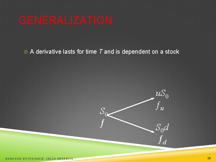
GENERALIZATION A derivative lasts for time T and is dependent on a stock S 0 ƒ BAHATTIN BUYUKSAHIN, CELSO BRUNETTI u. S 0 ƒu S 0 d ƒd 10

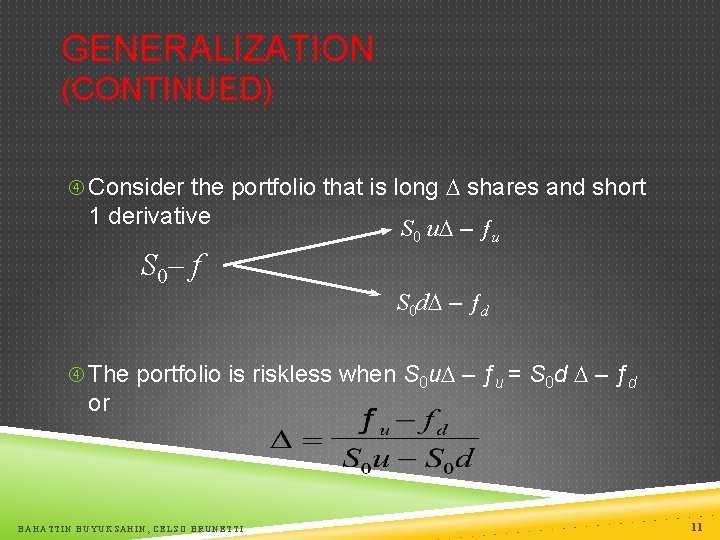
GENERALIZATION (CONTINUED) Consider the portfolio that is long shares and short 1 derivative S 0 u – ƒu S 0– f S 0 d – ƒd The portfolio is riskless when S 0 u – ƒu = S 0 d – ƒd or BAHATTIN BUYUKSAHIN, CELSO BRUNETTI 11

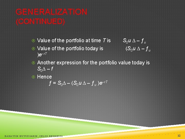
GENERALIZATION (CONTINUED) Value of the portfolio at time T is Value of the portfolio today is )e–r. T S 0 u – ƒu (S 0 u – ƒu Another expression for the portfolio value today is S 0 – f Hence ƒ = S 0 – (S 0 u – ƒu )e–r. T BAHATTIN BUYUKSAHIN, CELSO BRUNETTI 12

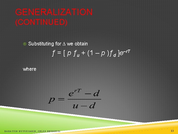
GENERALIZATION (CONTINUED) Substituting for we obtain ƒ = [ p ƒu + (1 – p )ƒd ]e–r. T where BAHATTIN BUYUKSAHIN, CELSO BRUNETTI 13

RISK-NEUTRAL VALUATION ƒ = [ p ƒu + (1 – p )ƒd ]e-r. T The variables p and (1 – p ) can be interpreted as the risk-neutral probabilities of up and down movements The value of a derivative is its expected payoff in a risk-neutral world discounted at the risk-free rate S 0 ƒ BAHATTIN BUYUKSAHIN, CELSO BRUNETTI (1 – p S 0 u ƒu p) S 0 d ƒd 14

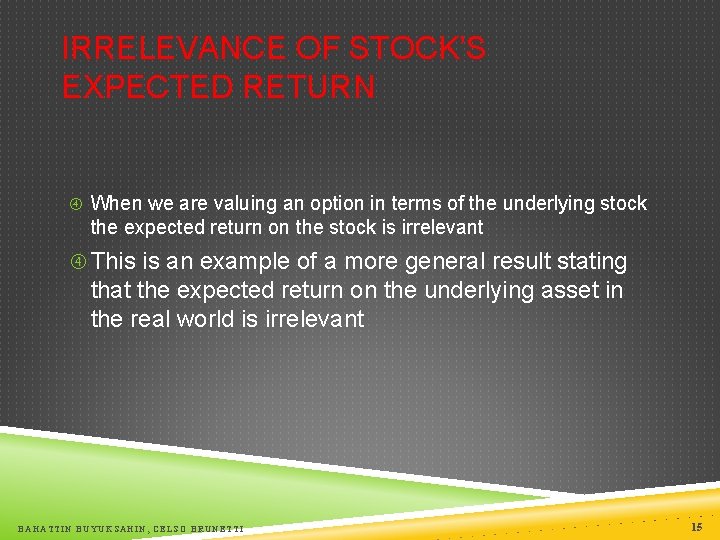
IRRELEVANCE OF STOCK’S EXPECTED RETURN When we are valuing an option in terms of the underlying stock the expected return on the stock is irrelevant This is an example of a more general result stating that the expected return on the underlying asset in the real world is irrelevant BAHATTIN BUYUKSAHIN, CELSO BRUNETTI 15

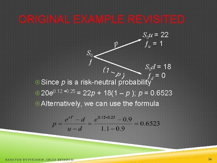
ORIGINAL EXAMPLE REVISITED p S 0 ƒ S 0 u = 22 ƒu = 1 S 0 d = 18 p) ƒd = 0 Since p is a risk-neutral probability 20 e 0. 12 *0. 25 = 22 p + 18(1 – p ); p = 0. 6523 Alternatively, we can use the formula BAHATTIN BUYUKSAHIN, CELSO BRUNETTI (1 – 16

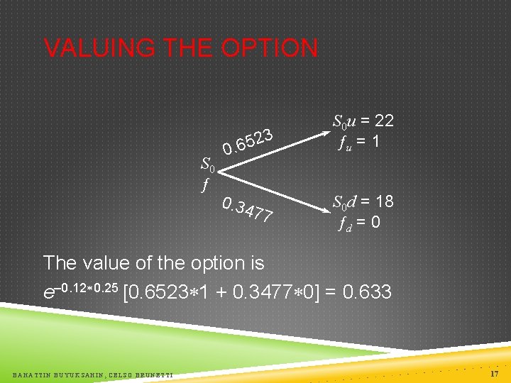
VALUING THE OPTION S 0 ƒ 3 2 5 0. 6 0. 34 77 S 0 u = 22 ƒu = 1 S 0 d = 18 ƒd = 0 The value of the option is e– 0. 12*0. 25 [0. 6523*1 + 0. 3477*0] = 0. 633 BAHATTIN BUYUKSAHIN, CELSO BRUNETTI 17

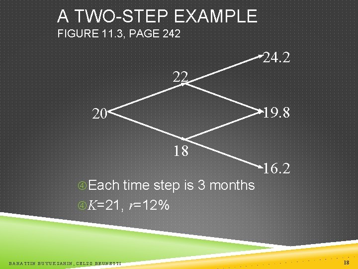
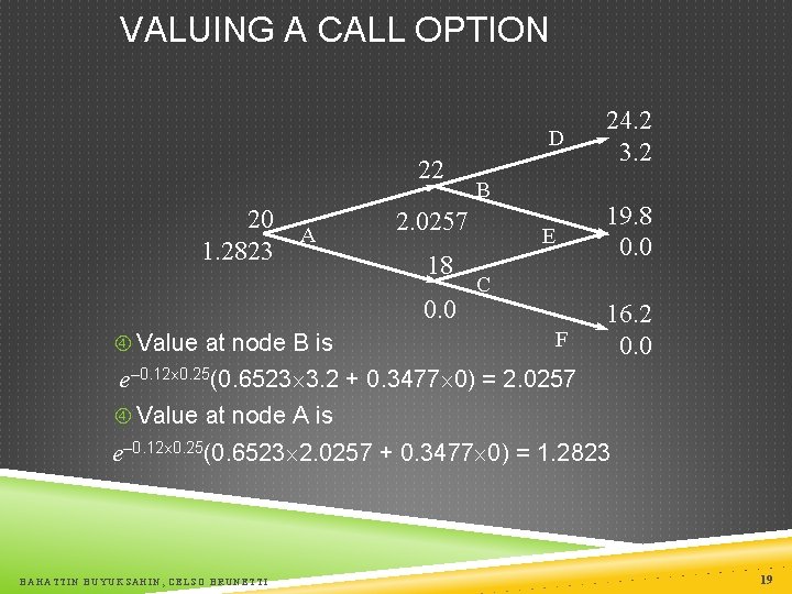
A TWO-STEP EXAMPLE FIGURE 11. 3, PAGE 242 24. 2 22 19. 8 20 18 16. 2 Each time step is 3 months K=21, r=12% BAHATTIN BUYUKSAHIN, CELSO BRUNETTI 18

VALUING A CALL OPTION D 22 20 1. 2823 A 2. 0257 18 0. 0 Value at node B is B E 24. 2 3. 2 19. 8 0. 0 C F 16. 2 0. 0 e– 0. 12´ 0. 25(0. 6523´ 3. 2 + 0. 3477´ 0) = 2. 0257 Value at node A is e– 0. 12´ 0. 25(0. 6523´ 2. 0257 + 0. 3477´ 0) = 1. 2823 BAHATTIN BUYUKSAHIN, CELSO BRUNETTI 19

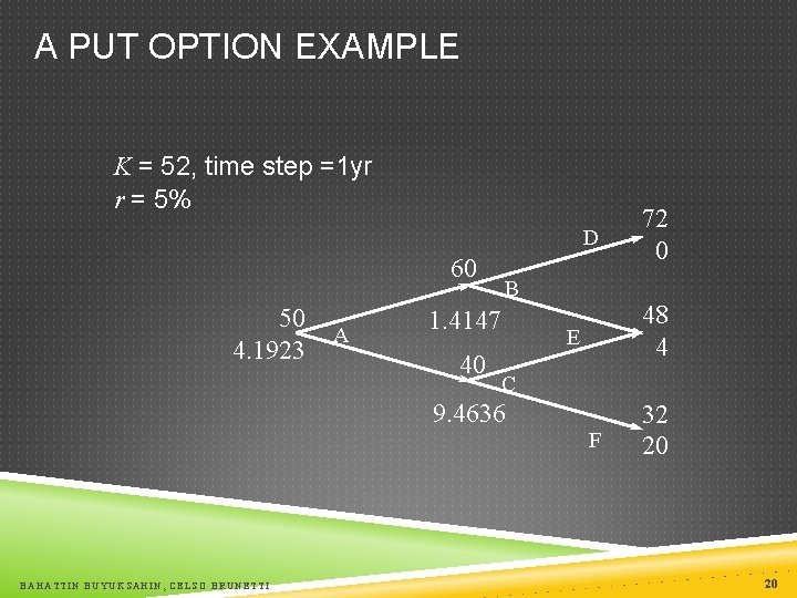
A PUT OPTION EXAMPLE K = 52, time step =1 yr r = 5% D 60 50 4. 1923 A B 1. 4147 40 48 4 E C 9. 4636 BAHATTIN BUYUKSAHIN, CELSO BRUNETTI 72 0 F 32 20 20

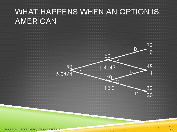
WHAT HAPPENS WHEN AN OPTION IS AMERICAN D 60 50 5. 0894 A 1. 4147 40 12. 0 BAHATTIN BUYUKSAHIN, CELSO BRUNETTI B 72 0 48 4 E C F 32 20 21

DELTA Delta ( ) is the ratio of the change in the price of a stock option to the change in the price of the underlying stock The value of varies from node to node BAHATTIN BUYUKSAHIN, CELSO BRUNETTI 22

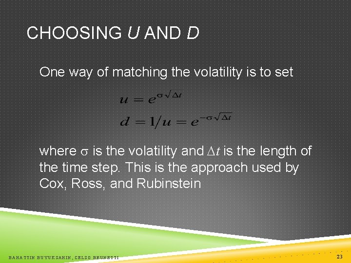
CHOOSING U AND D One way of matching the volatility is to set where s is the volatility and t is the length of the time step. This is the approach used by Cox, Ross, and Rubinstein BAHATTIN BUYUKSAHIN, CELSO BRUNETTI 23

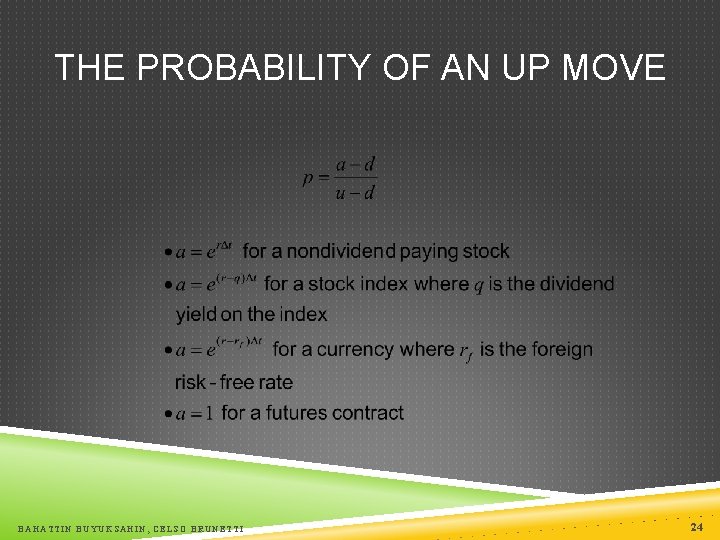
THE PROBABILITY OF AN UP MOVE BAHATTIN BUYUKSAHIN, CELSO BRUNETTI 24

THE BLACK-SCHOLES-MERTON MODEL

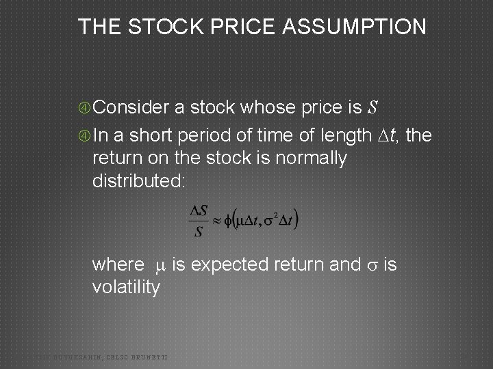
THE STOCK PRICE ASSUMPTION Consider a stock whose price is S In a short period of time of length t, the return on the stock is normally distributed: where is expected return and s is volatility BAHATTIN BUYUKSAHIN, CELSO BRUNETTI 26

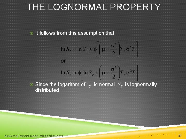
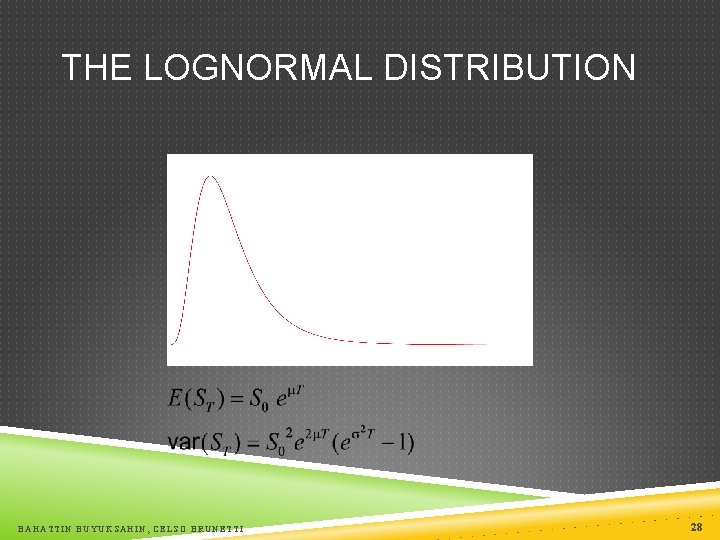
THE LOGNORMAL PROPERTY It follows from this assumption that Since the logarithm of ST is normal, ST is lognormally distributed BAHATTIN BUYUKSAHIN, CELSO BRUNETTI 27

THE LOGNORMAL DISTRIBUTION BAHATTIN BUYUKSAHIN, CELSO BRUNETTI 28

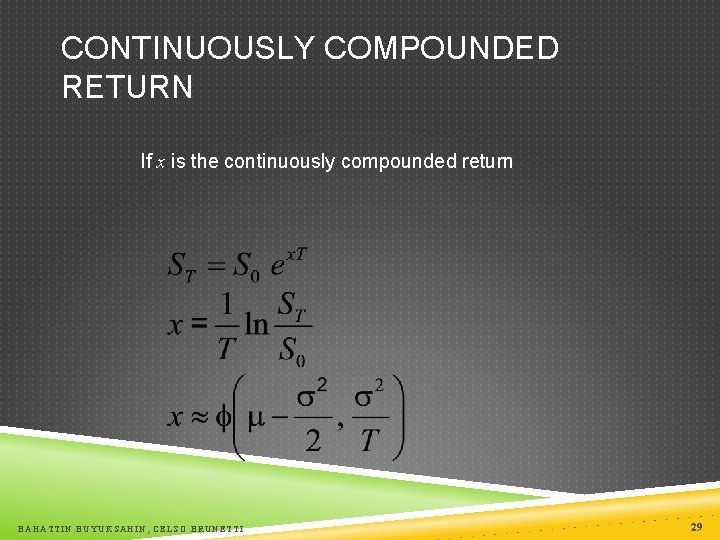
CONTINUOUSLY COMPOUNDED RETURN If x is the continuously compounded return BAHATTIN BUYUKSAHIN, CELSO BRUNETTI 29

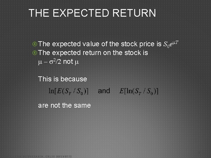
THE EXPECTED RETURN The expected value of the stock price is S 0 e T The expected return on the stock is – s 2/2 not This is because are not the same 30 BAHATTIN BUYUKSAHIN, CELSO BRUNETTI

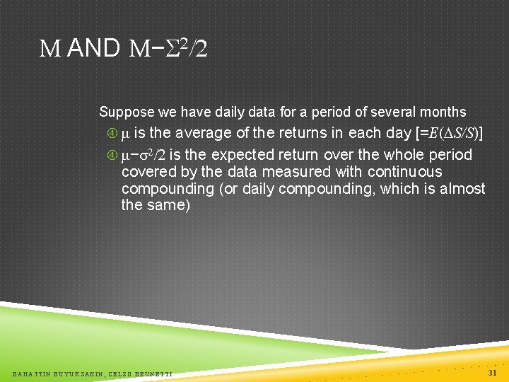
M AND M−S 2/2 Suppose we have daily data for a period of several months is the average of the returns in each day [=E( S/S)] −s 2/2 is the expected return over the whole period covered by the data measured with continuous compounding (or daily compounding, which is almost the same) BAHATTIN BUYUKSAHIN, CELSO BRUNETTI 31

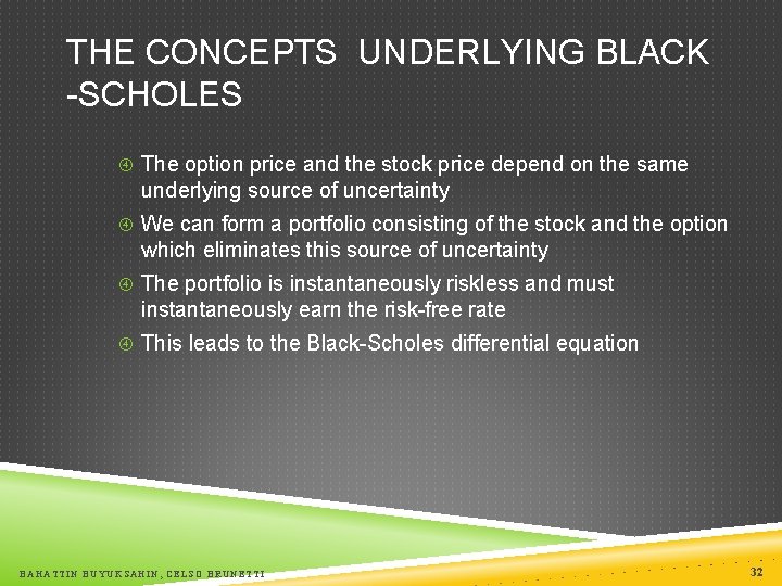
THE CONCEPTS UNDERLYING BLACK -SCHOLES The option price and the stock price depend on the same underlying source of uncertainty We can form a portfolio consisting of the stock and the option which eliminates this source of uncertainty The portfolio is instantaneously riskless and must instantaneously earn the risk-free rate This leads to the Black-Scholes differential equation BAHATTIN BUYUKSAHIN, CELSO BRUNETTI 32

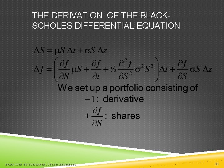
THE DERIVATION OF THE BLACKSCHOLES DIFFERENTIAL EQUATION BAHATTIN BUYUKSAHIN, CELSO BRUNETTI 33

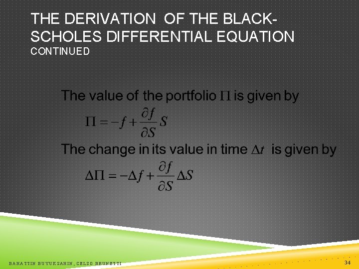
THE DERIVATION OF THE BLACKSCHOLES DIFFERENTIAL EQUATION CONTINUED BAHATTIN BUYUKSAHIN, CELSO BRUNETTI 34

THE DERIVATION OF THE BLACKSCHOLES DIFFERENTIAL EQUATION CONTINUED BAHATTIN BUYUKSAHIN, CELSO BRUNETTI 35

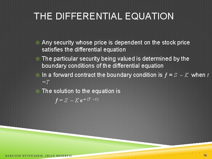
THE DIFFERENTIAL EQUATION Any security whose price is dependent on the stock price satisfies the differential equation The particular security being valued is determined by the boundary conditions of the differential equation In a forward contract the boundary condition is ƒ = S – K when t =T The solution to the equation is ƒ = S – K e–r (T BAHATTIN BUYUKSAHIN, CELSO BRUNETTI –t) 36

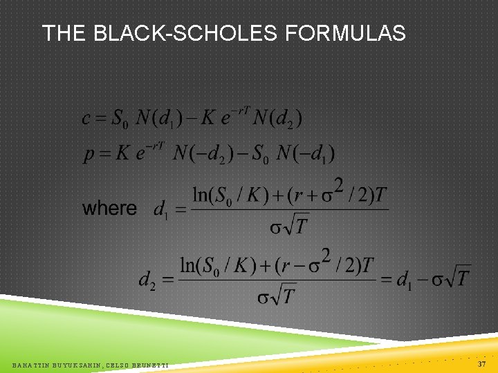
THE BLACK-SCHOLES FORMULAS BAHATTIN BUYUKSAHIN, CELSO BRUNETTI 37

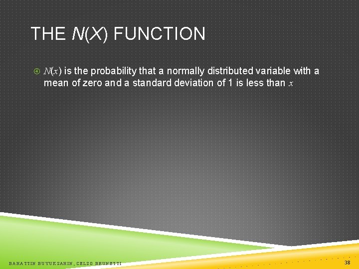
THE N(X) FUNCTION N(x) is the probability that a normally distributed variable with a mean of zero and a standard deviation of 1 is less than x BAHATTIN BUYUKSAHIN, CELSO BRUNETTI 38

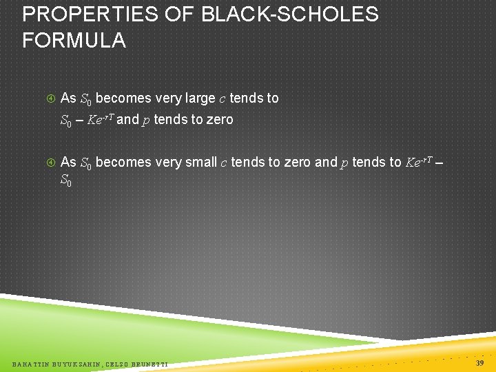
PROPERTIES OF BLACK-SCHOLES FORMULA As S 0 becomes very large c tends to S 0 – Ke-r. T and p tends to zero As S 0 becomes very small c tends to zero and p tends to Ke-r. T – S 0 BAHATTIN BUYUKSAHIN, CELSO BRUNETTI 39

RISK-NEUTRAL VALUATION The variable does not appear in the Black-Scholes equation The equation is independent of all variables affected by risk preference The solution to the differential equation is therefore the same in a risk-free world as it is in the real world This leads to the principle of risk-neutral valuation BAHATTIN BUYUKSAHIN, CELSO BRUNETTI 40

APPLYING RISK-NEUTRAL VALUATION 1. Assume that the expected return from the stock price is the risk-free rate 2. Calculate the expected payoff from the option 3. Discount at the risk-free rate BAHATTIN BUYUKSAHIN, CELSO BRUNETTI 41

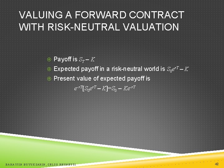
VALUING A FORWARD CONTRACT WITH RISK-NEUTRAL VALUATION Payoff is ST – K Expected payoff in a risk-neutral world is S 0 er. T – K Present value of expected payoff is e-r. T[S 0 er. T – K]=S 0 – Ke-r. T BAHATTIN BUYUKSAHIN, CELSO BRUNETTI 42

IMPLIED VOLATILITY The implied volatility of an option is the volatility for which the Black-Scholes price equals the market price There is a one-to-one correspondence between prices and implied volatilities Traders and brokers often quote implied volatilities rather than dollar prices BAHATTIN BUYUKSAHIN, CELSO BRUNETTI 43

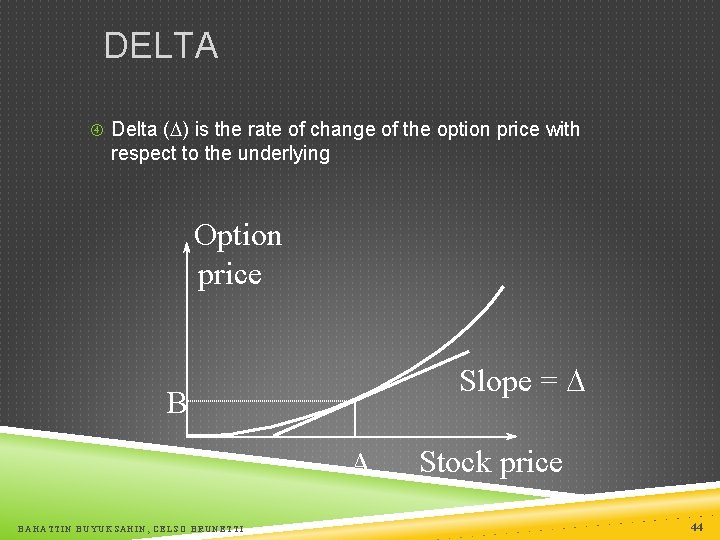
DELTA Delta ( ) is the rate of change of the option price with respect to the underlying Option price Slope = B A BAHATTIN BUYUKSAHIN, CELSO BRUNETTI Stock price 44

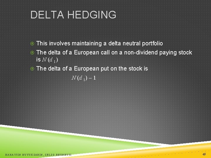
DELTA HEDGING This involves maintaining a delta neutral portfolio The delta of a European call on a non-dividend paying stock is N (d 1) The delta of a European put on the stock is N (d 1) – 1 BAHATTIN BUYUKSAHIN, CELSO BRUNETTI 45

DELTA HEDGING CONTINUED The hedge position must be frequently rebalanced Delta hedging a written option involves a “buy high, sell low” trading rule BAHATTIN BUYUKSAHIN, CELSO BRUNETTI 46

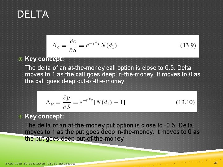
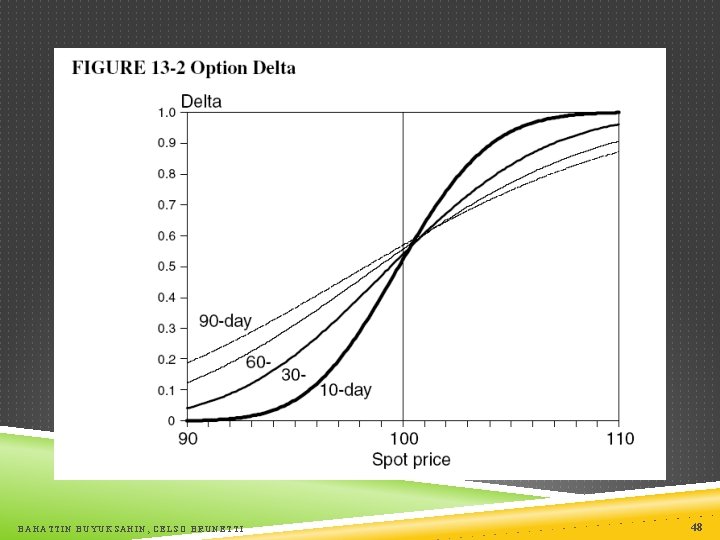
DELTA Key concept: The delta of an at-the-money call option is close to 0. 5. Delta moves to 1 as the call goes deep in-the-money. It moves to 0 as the call goes deep out-of-the-money Key concept: The delta of an at-the-money put option is close to -0. 5. Delta moves to 1 as the put goes deep in-the-money. It moves to 0 as the put goes deep out-of-the-money BAHATTIN BUYUKSAHIN, CELSO BRUNETTI 47

BAHATTIN BUYUKSAHIN, CELSO BRUNETTI 48

THETA � Theta ( ) of a derivative (or portfolio of derivatives) is the rate of change of the value with respect to the passage of time � The theta of a call or put is usually negative. This means that, if time passes with the price of the underlying asset and its volatility remaining the same, the value of a long option declines BAHATTIN BUYUKSAHIN, CELSO BRUNETTI 49

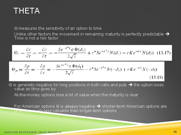
THETA measures the sensitivity of an option to time Unlike other factors the movement in remaining maturity is perfectly predictable Time is not a risk factor is generally negative for long positions in both calls and puts the option loses value as time goes by At-the-money options lose a lot of value when the maturity is near For American options is always negative shorter-term American options are unambiguously less valuable than longer-term options BAHATTIN BUYUKSAHIN, CELSO BRUNETTI 50

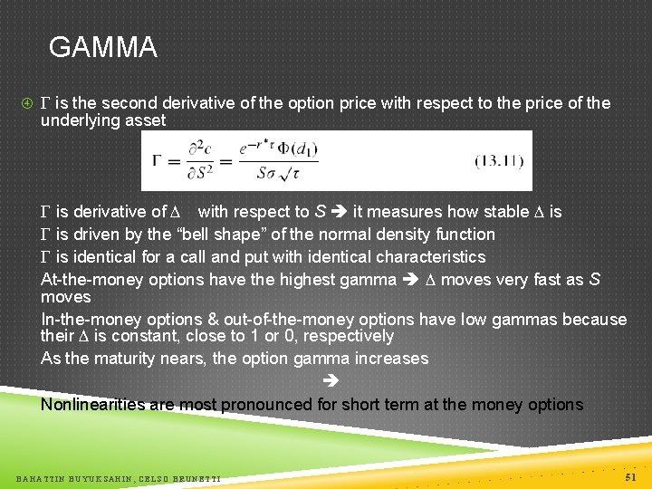
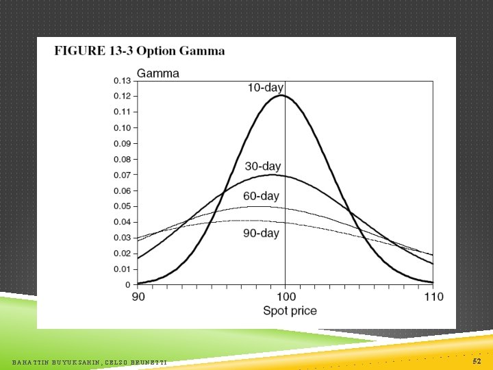
GAMMA is the second derivative of the option price with respect to the price of the underlying asset is derivative of with respect to S it measures how stable is driven by the “bell shape” of the normal density function is identical for a call and put with identical characteristics At-the-money options have the highest gamma moves very fast as S moves In-the-money options & out-of-the-money options have low gammas because their is constant, close to 1 or 0, respectively As the maturity nears, the option gamma increases Nonlinearities are most pronounced for short term at the money options BAHATTIN BUYUKSAHIN, CELSO BRUNETTI 51

BAHATTIN BUYUKSAHIN, CELSO BRUNETTI 52

GAMMA for options is similar to the concept of convexity for bonds Bonds usually have positive convexity, whereas options can create positive or negative Positive convexity or is beneficial the value of the asset drops more slowly and increase more quickly when the market risk factor moves Negative convexity and can be dangerous because it implies faster price falls and slower price increases Long positions in options, whether calls or puts, create positive convexity Short positions create negative convexity In exchange for assuming the harmful effect of this negative convexity, option sellers receive the premium BAHATTIN BUYUKSAHIN, CELSO BRUNETTI 53

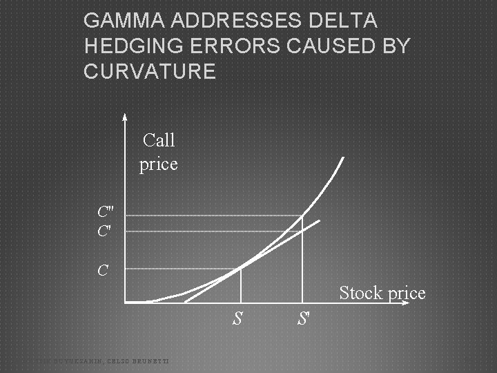
GAMMA ADDRESSES DELTA HEDGING ERRORS CAUSED BY CURVATURE Call price C'' C' C Stock price S BAHATTIN BUYUKSAHIN, CELSO BRUNETTI S' 54

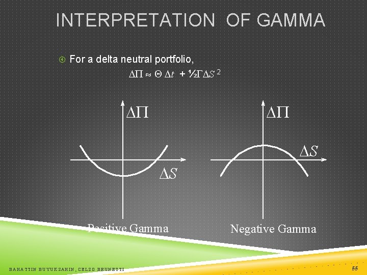
INTERPRETATION OF GAMMA For a delta neutral portfolio, P » t + ½ S 2 P P S S Positive Gamma BAHATTIN BUYUKSAHIN, CELSO BRUNETTI Negative Gamma 55

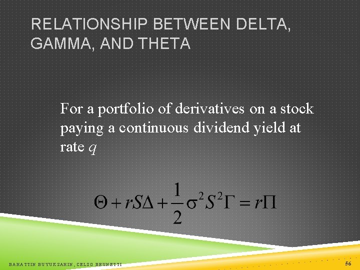
RELATIONSHIP BETWEEN DELTA, GAMMA, AND THETA For a portfolio of derivatives on a stock paying a continuous dividend yield at rate q BAHATTIN BUYUKSAHIN, CELSO BRUNETTI 56

VEGA Vega ( n) is the rate of change of the value of a derivatives portfolio with respect to volatility Vega tends to be greatest for options that are close to the money BAHATTIN BUYUKSAHIN, CELSO BRUNETTI 57

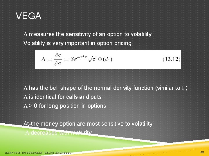
VEGA measures the sensitivity of an option to volatility Volatility is very important in option pricing has the bell shape of the normal density function (similar to ) is identical for calls and puts > 0 for long position in options At-the money option are most sensitive to volatility decreases with maturity BAHATTIN BUYUKSAHIN, CELSO BRUNETTI 58

MANAGING DELTA, GAMMA, & VEGA · can be changed by taking a position in the underlying To adjust & n it is necessary to take a position in an option or other derivative BAHATTIN BUYUKSAHIN, CELSO BRUNETTI 59

RHO Rho is the rate of change of the value of a derivative with respect to the interest rate BAHATTIN BUYUKSAHIN, CELSO BRUNETTI 60

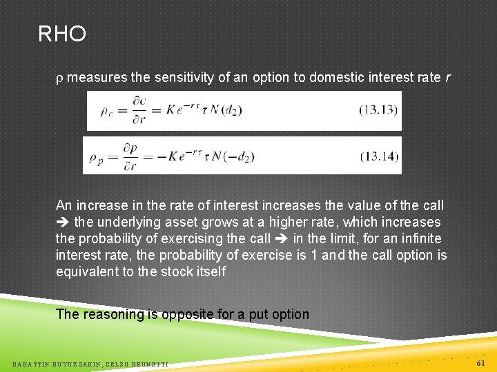
RHO measures the sensitivity of an option to domestic interest rate r An increase in the rate of interest increases the value of the call the underlying asset grows at a higher rate, which increases the probability of exercising the call in the limit, for an infinite interest rate, the probability of exercise is 1 and the call option is equivalent to the stock itself The reasoning is opposite for a put option BAHATTIN BUYUKSAHIN, CELSO BRUNETTI 61

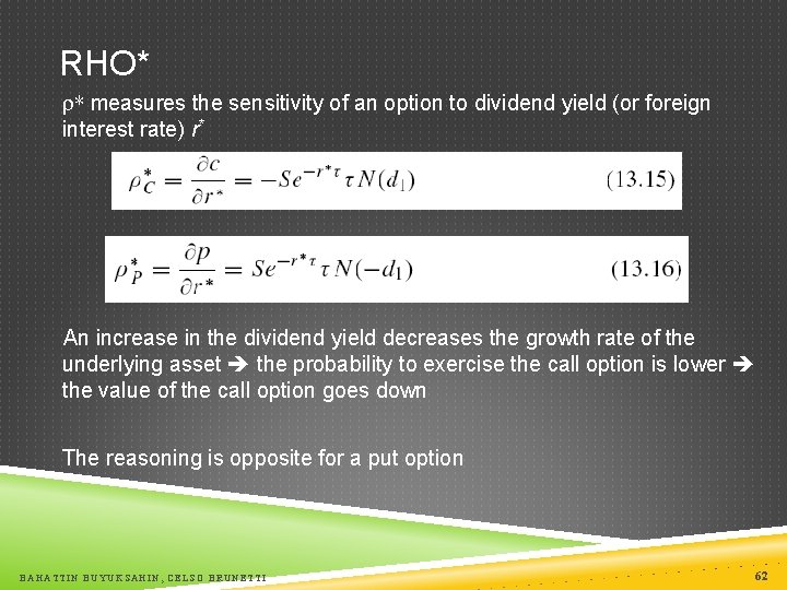
RHO* * measures the sensitivity of an option to dividend yield (or foreign interest rate) r* An increase in the dividend yield decreases the growth rate of the underlying asset the probability to exercise the call option is lower the value of the call option goes down The reasoning is opposite for a put option BAHATTIN BUYUKSAHIN, CELSO BRUNETTI 62

HEDGING IN PRACTICE Traders usually ensure that their portfolios are delta-neutral at least once a day Whenever the opportunity arises, they improve gamma and vega As portfolio becomes larger hedging becomes less expensive BAHATTIN BUYUKSAHIN, CELSO BRUNETTI 63

SCENARIO ANALYSIS A scenario analysis involves testing the effect on the value of a portfolio of different assumptions concerning asset prices and their volatilities BAHATTIN BUYUKSAHIN, CELSO BRUNETTI 64

FUTURES CONTRACT CAN BE USED FOR HEDGING The delta of a futures contract on an asset paying a yield at rate q is e(r-q)T times the delta of a spot contract The position required in futures for delta hedging is therefore e-(rq)T times the position required in the corresponding spot contract BAHATTIN BUYUKSAHIN, CELSO BRUNETTI 65

HEDGING VS CREATION OF AN OPTION SYNTHETICALLY When we are hedging we take positions that offset , , n, etc. When we create an option synthetically we take positions that match , , & BAHATTIN BUYUKSAHIN, CELSO BRUNETTI n 66

PORTFOLIO INSURANCE In October of 1987 many portfolio managers attempted to create a put option on a portfolio synthetically This involves initially selling enough of the portfolio (or of index futures) to match the of the put option BAHATTIN BUYUKSAHIN, CELSO BRUNETTI 67

PORTFOLIO INSURANCE CONTINUED As the value of the portfolio increases, the of the put becomes less negative and some of the original portfolio is repurchased As the value of the portfolio decreases, the of the put becomes more negative and more of the portfolio must be sold BAHATTIN BUYUKSAHIN, CELSO BRUNETTI 68

PORTFOLIO INSURANCE CONTINUED The strategy did not work well on October 19, 1987. . . BAHATTIN BUYUKSAHIN, CELSO BRUNETTI 69

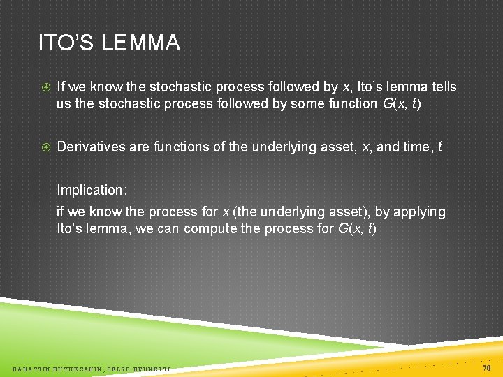
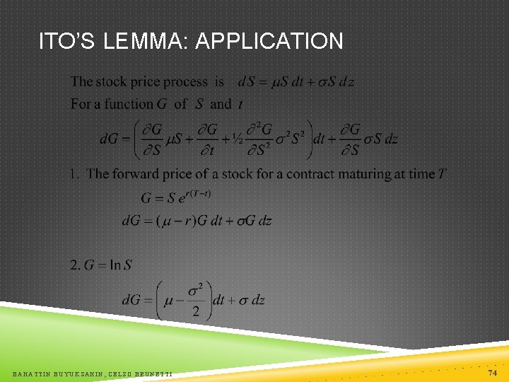
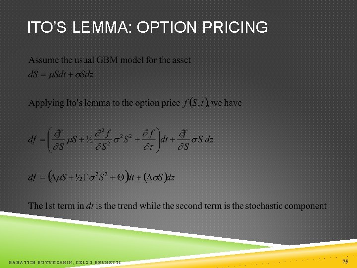
ITO’S LEMMA If we know the stochastic process followed by x, Ito’s lemma tells us the stochastic process followed by some function G(x, t) Derivatives are functions of the underlying asset, x, and time, t Implication: if we know the process for x (the underlying asset), by applying Ito’s lemma, we can compute the process for G(x, t) BAHATTIN BUYUKSAHIN, CELSO BRUNETTI 70

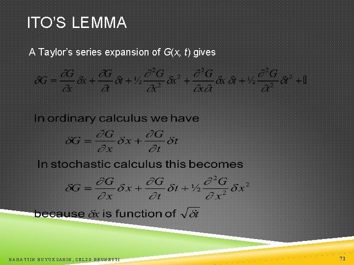
ITO’S LEMMA A Taylor’s series expansion of G(x, t) gives BAHATTIN BUYUKSAHIN, CELSO BRUNETTI 71

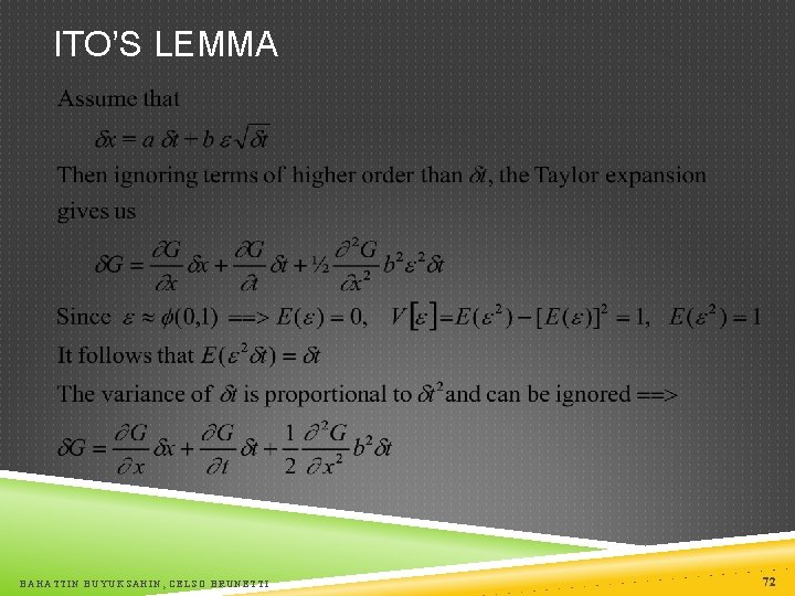
ITO’S LEMMA BAHATTIN BUYUKSAHIN, CELSO BRUNETTI 72

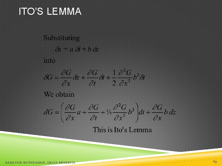
ITO’S LEMMA BAHATTIN BUYUKSAHIN, CELSO BRUNETTI 73

ITO’S LEMMA: APPLICATION BAHATTIN BUYUKSAHIN, CELSO BRUNETTI 74

ITO’S LEMMA: OPTION PRICING BAHATTIN BUYUKSAHIN, CELSO BRUNETTI 75

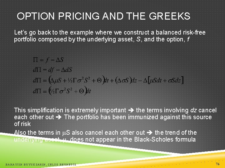
OPTION PRICING AND THE GREEKS Let’s go back to the example where we construct a balanced risk-free portfolio composed by the underlying asset, S, and the option, f This simplification is extremely important the terms involving dz cancel each other out The portfolio has been immunized against this source of risk Also the terms in S also cancel each other out the trend of the underlying asset, , does not appear in the Black-Scholes formula BAHATTIN BUYUKSAHIN, CELSO BRUNETTI 76

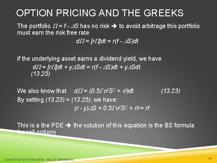
OPTION PRICING AND THE GREEKS The portfolio = f - S has no risk to avoid arbitrage this portfolio must earn the risk free rate d = [r ]dt = r(f - S)dt if the underlying asset earns a dividend yield, we have d = [r ]dt + y Sdt = r(f - S)dt + y Sdt (13. 25) We also know that d = (0. 5 2 S 2 + )dt By setting (13. 23) = (13. 25), we have: (r - y) S + 0. 5 2 S 2 + = rf (13. 23) This is a the PDE the solution of this equation is the BS formula for call options BAHATTIN BUYUKSAHIN, CELSO BRUNETTI 77

BAHATTIN BUYUKSAHIN, CELSO BRUNETTI 78

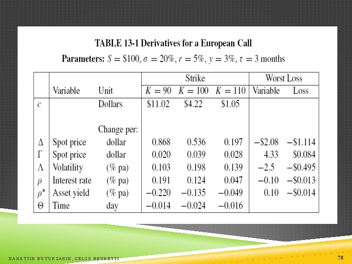
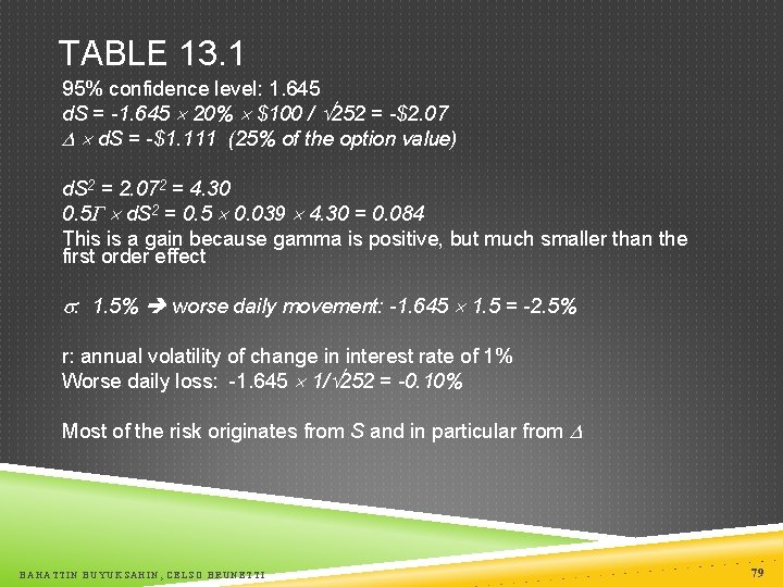
TABLE 13. 1 95% confidence level: 1. 645 d. S = -1. 645 20% $100 / 252 = -$2. 07 d. S = -$1. 111 (25% of the option value) d. S 2 = 2. 072 = 4. 30 0. 5 d. S 2 = 0. 5 0. 039 4. 30 = 0. 084 This is a gain because gamma is positive, but much smaller than the first order effect : 1. 5% worse daily movement: -1. 645 1. 5 = -2. 5% r: annual volatility of change in interest rate of 1% Worse daily loss: -1. 645 1/ 252 = -0. 10% Most of the risk originates from S and in particular from BAHATTIN BUYUKSAHIN, CELSO BRUNETTI 79

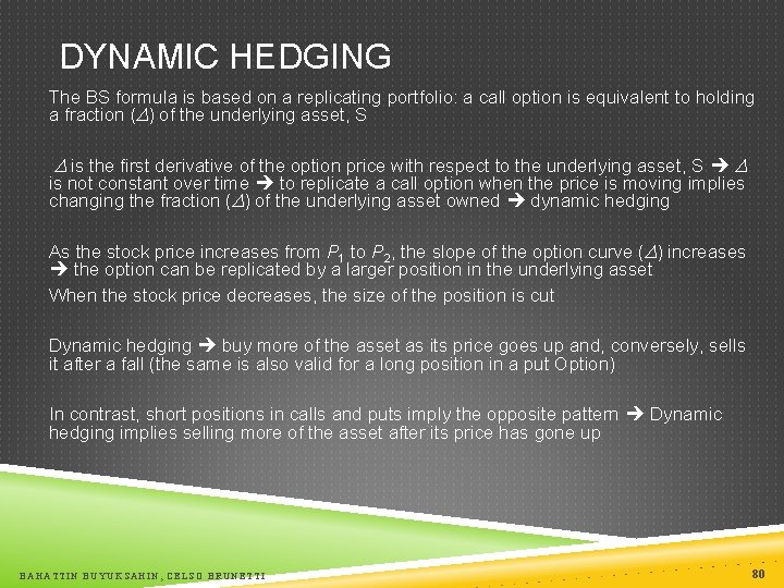
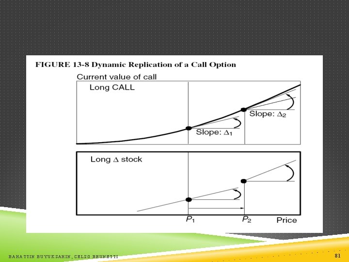
DYNAMIC HEDGING The BS formula is based on a replicating portfolio: a call option is equivalent to holding a fraction ( ) of the underlying asset, S is the first derivative of the option price with respect to the underlying asset, S is not constant over time to replicate a call option when the price is moving implies changing the fraction ( ) of the underlying asset owned dynamic hedging As the stock price increases from P 1 to P 2, the slope of the option curve ( ) increases the option can be replicated by a larger position in the underlying asset When the stock price decreases, the size of the position is cut Dynamic hedging buy more of the asset as its price goes up and, conversely, sells it after a fall (the same is also valid for a long position in a put Option) In contrast, short positions in calls and puts imply the opposite pattern Dynamic hedging implies selling more of the asset after its price has gone up BAHATTIN BUYUKSAHIN, CELSO BRUNETTI 80

BAHATTIN BUYUKSAHIN, CELSO BRUNETTI 81

INTERESTING QUESTION Shall we rebalance our portfolio every time the price move? Be careful!!! BAHATTIN BUYUKSAHIN, CELSO BRUNETTI 82

DISTRIBUTION OF OPTION PAYOFFS Unlike linear derivatives such as forwards and futures, payoffs on options are asymmetric This is not necessarily because of the distribution of the underlying factor, which is often symmetric Long positions in options, whether calls or puts, have positive gamma, positive skewness, or long right tails Short positions in options are short gamma and hence have negative skewness or long left tails BAHATTIN BUYUKSAHIN, CELSO BRUNETTI 83

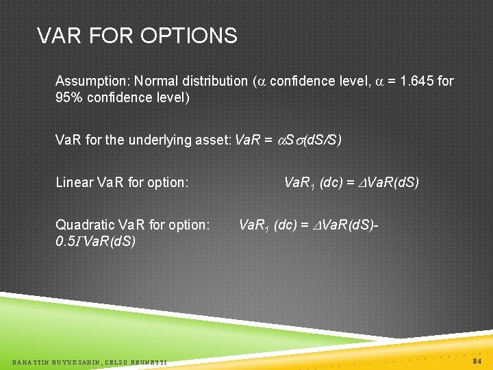
VAR FOR OPTIONS Assumption: Normal distribution ( confidence level, = 1. 645 for 95% confidence level) Va. R for the underlying asset: Va. R = S (d. S/S) Linear Va. R for option: Quadratic Va. R for option: 0. 5 Va. R(d. S) BAHATTIN BUYUKSAHIN, CELSO BRUNETTI Va. R 1 (dc) = Va. R(d. S)- 84

VAR FOR OPTIONS In computing Va. R for options it is important the nonlinearity of the option payoffs The degree of nonlinearity depends on the horizon With a Va. R horizon of two weeks, the range of possible values for S is quite narrow If S follows a normal distribution, the option value will be approximately normal If the VAR horizon is set at two months, the nonlinearities in the exposure combine with the greater range of price movements create a heavily skewed distribution So for plain-vanilla options, the linear approximation may be adequate as long as the Va. R horizon is kept short For more exotic options, or longer VAR horizons, the risk manager needs to account for nonlinearities BAHATTIN BUYUKSAHIN, CELSO BRUNETTI 85