Hebb Algorithm Hebb algorithm We consider the training

Hebb Algorithm

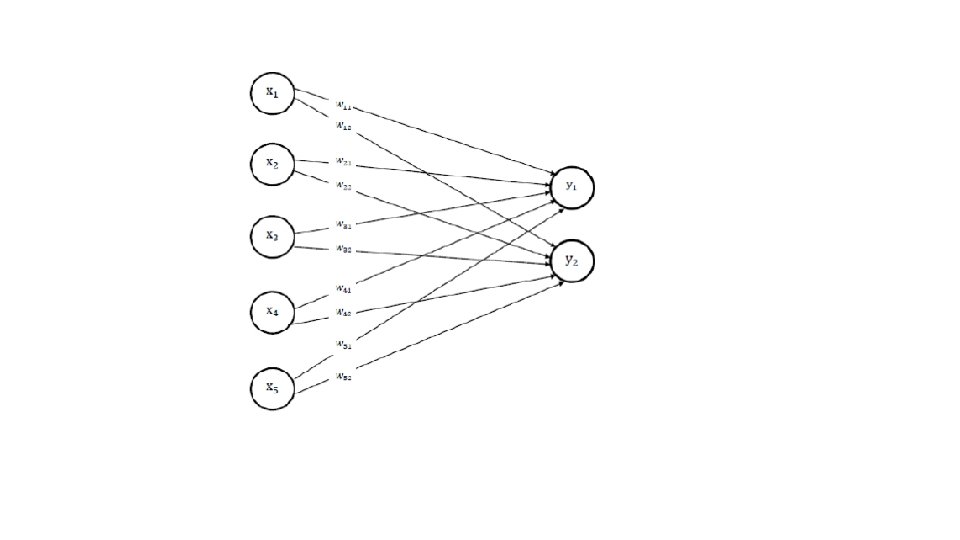
Hebb algorithm • We consider the training pair of vectors inputs – output • A = {a 1, a 2, . . }, output B={b 1, b 2, …} • Set all the initial weights equal to 0: Wij = 0 • Adjust weights wnew = w old + ab • We write the training vector of the matrix product as a column represented as n x 1 matrix and the target vector represented as a row vector with 1 x m matrix

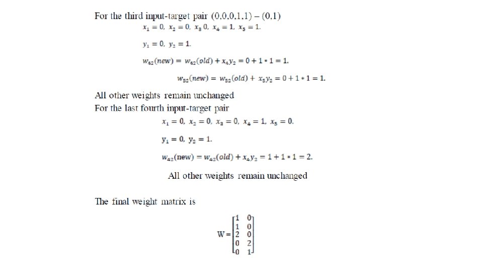
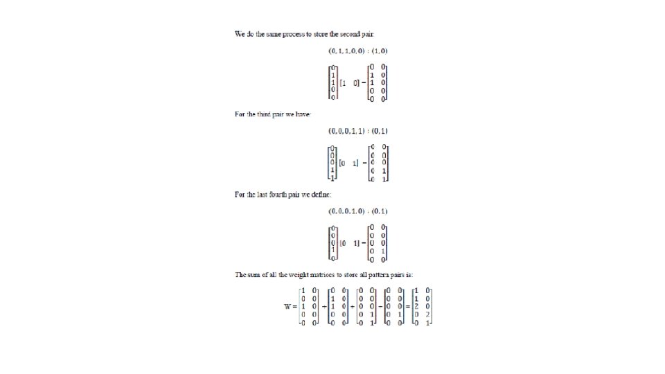
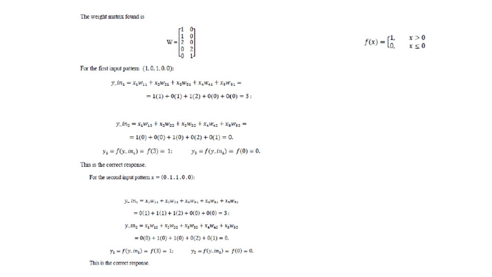
• we can find the weight matrix to store the association A, B • EXAMPLE First input A = (1, 0, 0) target t=(1, 0) Second input A = (0, 1, 1, 0, 0) target t=(1, 0) Third input A = (0, 0, 0, 1, 1) target t=(0, 1) Fourth Input A = (0, 0, 0, 1, 0) target t=(0, 1)

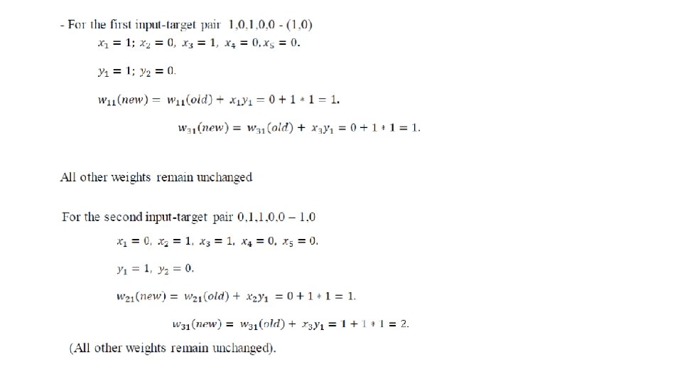
Let’s now use outer products instead of the algorithm of the Hebb rule. • Using outer product leads to the same weights which were found by the application of the Hebb rule. For the first input-target pair

test

AND gate using hebb

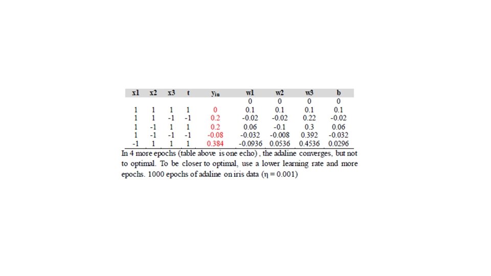
• Adaline Learning Rule Let η be the learning rate, and d the desired (target) real number output o. The learning rule is: w = w + η (d − o)x The weighted sum u is a dot product: u = w · x = Σ������ =1 Simple ADELINE for Pattern Classi_cation The learning rule is also called the LMS (least mean square) algorithm and the Widrow-Hoff learning rule. Approximately, the adaline converges to least squares (L 2) error Adaline Example (η = 0. 1) , d is target yin= b+x 1 w 1+x 2 w 2+x 3 w 3 wnew = wold +. 1(t-yin)xi bnew= wold +. 1(t-yin) Error = (t-yin)2