Health and Development 1 Health and development An

Health and Development 1

Health and development • An observation: health and wealth are correlated both across countries and across people within societies. Why? • Question #1: What is the impact of income on health and nutrition? • Question #2: What is the impact of health/nutrition on economic outcomes? • Question #3: Which policies / institutions improve the delivery of public health services in poor countries? 2

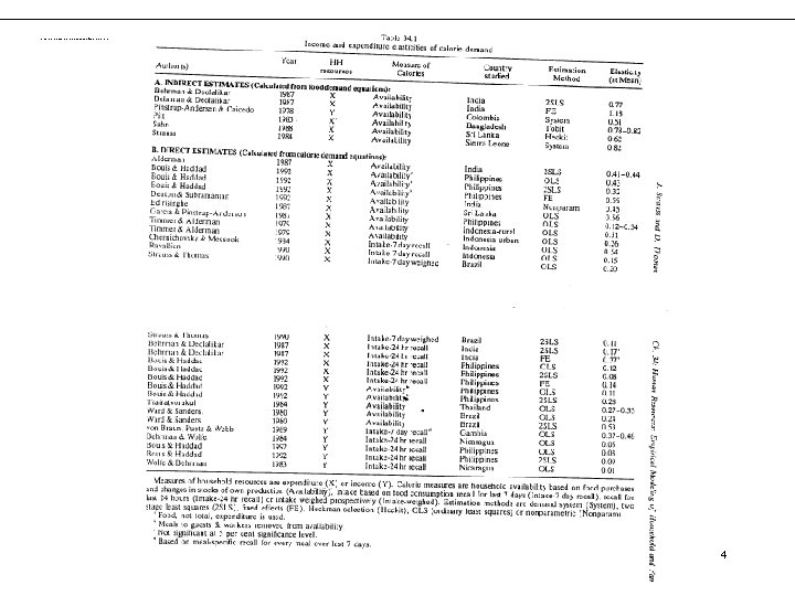
The health-wealth relationship • Disentangling the relationships between health and wealth and uncovering causal relationships in either direction is very tricky – Fundamental endogeneity problem – Measurement issues – Health: inputs (nutrition, expenditure) or output (health status) – Proper measurement of inputs: adjustment for quality, wastage – Wealth: short or long run? Measurement error in income – Functional form: non-linearities are key to the story, but it may not be possible to observe them • Table 1 (Strauss and Thomas): Wide variety in the estimates of the elasticities of calorie demand with respect to household resources (0. 01 to 0. 82) 3

Income and expenditure elasticities of calorie demand 4

Deaton and Subramanian (1996) • Nonparametric approach to examining the impact of wealth on health • Data set: 5, 630 households in 563 villages • Recall data on 149 food items, meals taken out and given away, etc. – From those 149 food items, they calculate caloric intake using a conversion table. Also correct for meals taken out and meals given to people. • Interesting aspect of this work: non-parametric estimates y = g(x) + e • How can we estimate g(x)? – Kernel regression – Fan (1992) locally weighted regression 5

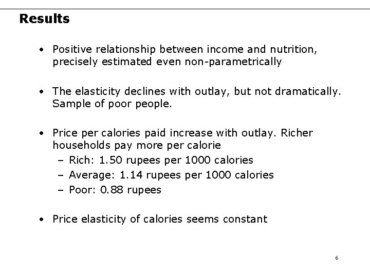
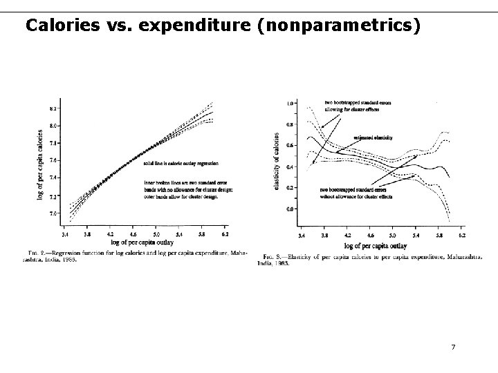
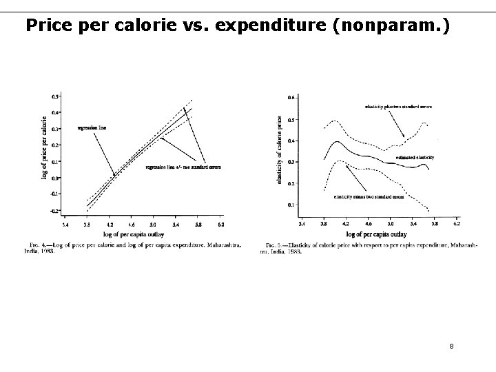
Results • Positive relationship between income and nutrition, precisely estimated even non-parametrically • The elasticity declines with outlay, but not dramatically. Sample of poor people. • Price per calories paid increase with outlay. Richer households pay more per calorie – Rich: 1. 50 rupees per 1000 calories – Average: 1. 14 rupees per 1000 calories – Poor: 0. 88 rupees • Price elasticity of calories seems constant 6

Calories vs. expenditure (nonparametrics) 7

Price per calorie vs. expenditure (nonparam. ) 8

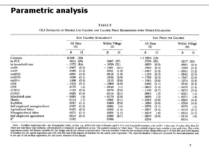
Parametric analysis 9

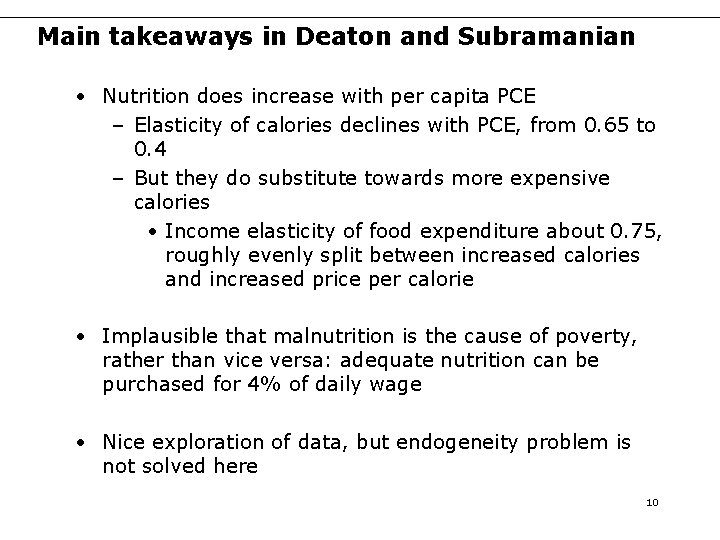
Main takeaways in Deaton and Subramanian • Nutrition does increase with per capita PCE – Elasticity of calories declines with PCE, from 0. 65 to 0. 4 – But they do substitute towards more expensive calories • Income elasticity of food expenditure about 0. 75, roughly evenly split between increased calories and increased price per calorie • Implausible that malnutrition is the cause of poverty, rather than vice versa: adequate nutrition can be purchased for 4% of daily wage • Nice exploration of data, but endogeneity problem is not solved here 10

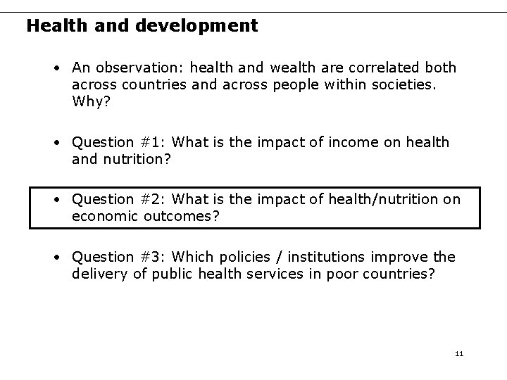
Health and development • An observation: health and wealth are correlated both across countries and across people within societies. Why? • Question #1: What is the impact of income on health and nutrition? • Question #2: What is the impact of health/nutrition on economic outcomes? • Question #3: Which policies / institutions improve the delivery of public health services in poor countries? 11

Under the Weather: Health, Schooling, and Socioeconomic Consequences of Early-Life Rainfall Sharon Maccini University of Michigan Dean Yang University of Michigan 12

Motivation • Life in rural areas of developing countries is prone to many kinds of risk • In addition to short-run effects, consequences of certain shocks may be felt many years or even decades later – Important for targeting of public resources that help cushion impact of shocks • Health shocks at the earliest stages of life, by affecting long-run health human capital, may have effects that extend into adulthood 13

Pigs 14

This paper … • Examines the long-run impact of exogenous environmental shocks in early life – Rainfall shocks in locality and year of birth, for Indonesian adults – Health as well as socioeconomic outcomes • Compares long-run impact of shocks experienced at different points in early life – Tests for the existence of “critical periods” in child development • Provides suggestive evidence on the pathways through which early-life rainfall affects adult outcomes 15

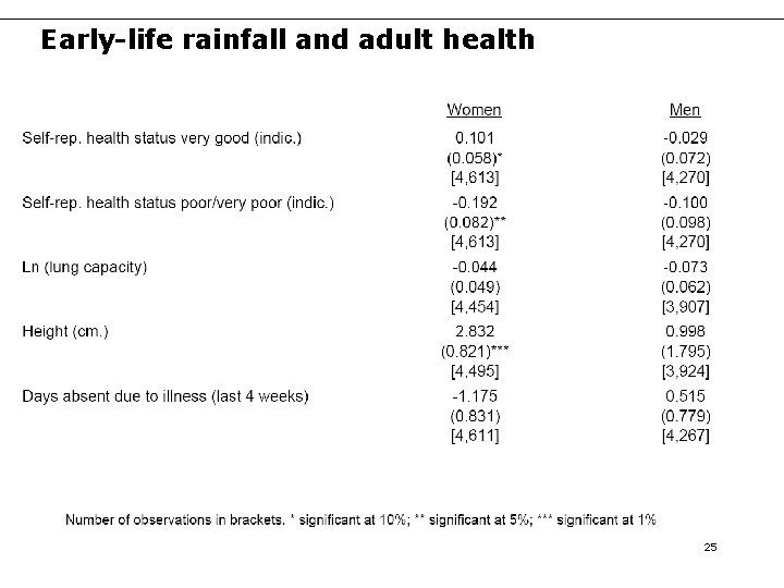
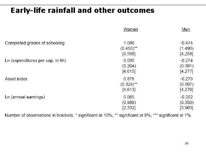
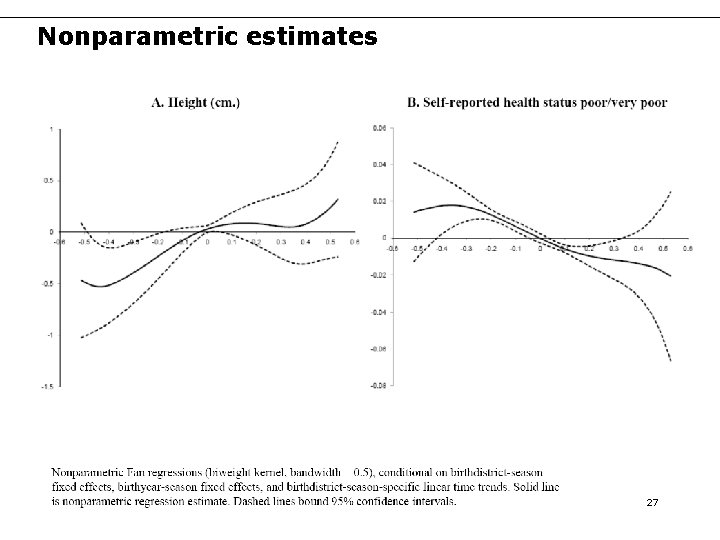
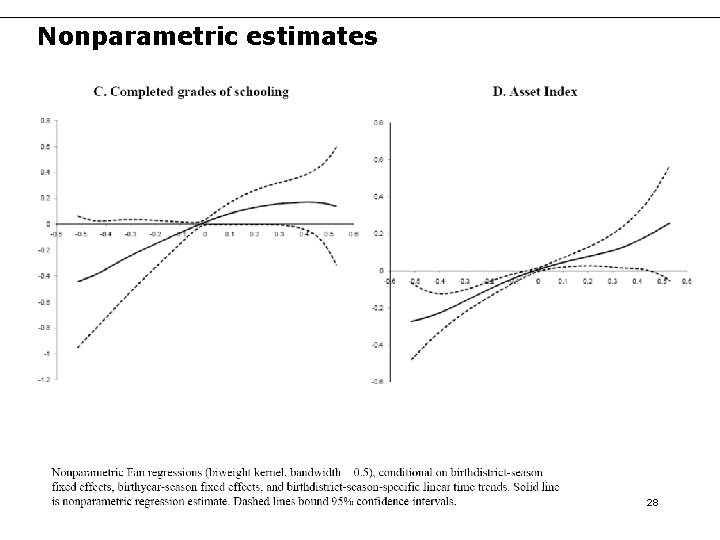
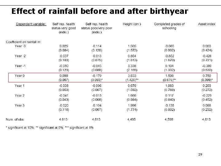
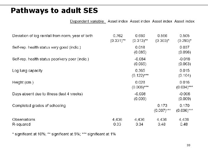
Summary of results • For women, 20% higher birthyear rainfall leads to: – Better health: 0. 57 centimeters greater height, 3. 8 percentage points less likely to report poor/very poor health – More education: 0. 22 more completed grades of schooling – Improved socioeconomic status: 0. 12 standard deviation higher asset index in household • No corresponding effects for men, possibly due to gender bias in household resource allocation in hard times • Rainfall in the first year of life has greatest effect on adult outcomes • Evidence consistent with the following chain of causation: Early-life rainfall infant health schooling adult SES 16

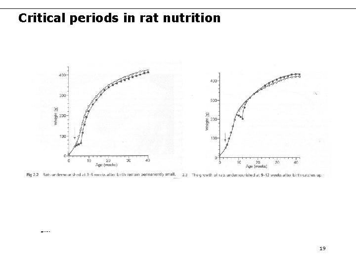
Critical-period programming • Exposure to certain stimuli during a sensitive time span may have irreversible effects on living organisms • “Fetal origins hypothesis”: The fetal stage and infancy are critical periods in human physical development – Early-life shocks can have long-lasting effects on health (Barker 1998) • Faced with poor nutrition/health conditions, limited resources prioritized for brain, compromising physical growth and development of other organ systems – Individuals are “programmed” for smaller body size, worse health later in life • Evidence: – Animal studies (see figures) – Epidemiological research in human populations • But causality often questionable 17

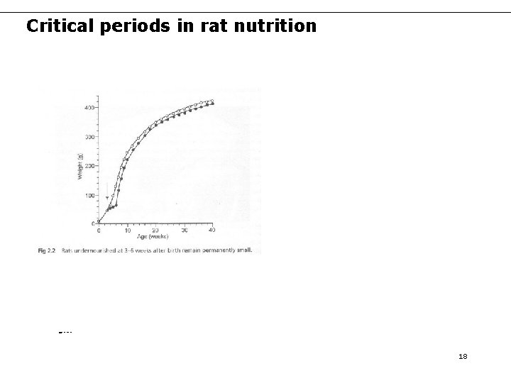
Critical periods in rat nutrition Source : Figures 2. 2 and 2. 3, Barker (1998) 18

Critical periods in rat nutrition Source : Figures 2. 2 and 2. 3, Barker (1998) 19

Identifying the impact of early-life shocks • Relater life outcomes to early-life health conditions – e. g. , cross-sectional differences in birthplace infant mortality, individual self-reported health status Open to omitted variable concerns • Examine impact of shocks to health conditions at birth – e. g. , within-twin birthweight differences, epidemics Difficult to generalize results from unusual events Data often a serious limitation • We examine impact of an important source of environmental variation in developing countries: rainfall – Using high-quality survey data in IFLS 20

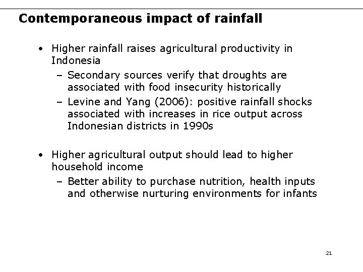
Contemporaneous impact of rainfall • Higher rainfall raises agricultural productivity in Indonesia – Secondary sources verify that droughts are associated with food insecurity historically – Levine and Yang (2006): positive rainfall shocks associated with increases in rice output across Indonesian districts in 1990 s • Higher agricultural output should lead to higher household income – Better ability to purchase nutrition, health inputs and otherwise nurturing environments for infants 21

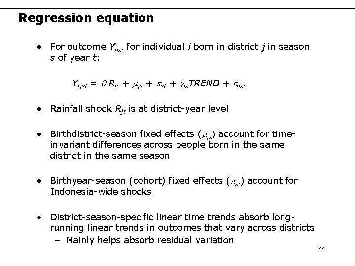
Regression equation • For outcome Yijst for individual i born in district j in season s of year t: Yijst = q Rjt + mjs + pst + gjs. TREND + eijst • Rainfall shock Rjt is at district-year level • Birthdistrict-season fixed effects (mjs) account for timeinvariant differences across people born in the same district in the same season • Birthyear-season (cohort) fixed effects (pst) account for Indonesia-wide shocks • District-season-specific linear time trends absorb longrunning linear trends in outcomes that vary across districts – Mainly helps absorb residual variation 22

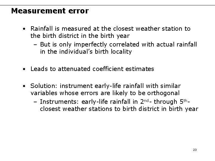
Measurement error • Rainfall is measured at the closest weather station to the birth district in the birth year – But is only imperfectly correlated with actual rainfall in the individual’s birth locality • Leads to attenuated coefficient estimates • Solution: instrument early-life rainfall with similar variables whose errors are likely to be orthogonal – Instruments: early-life rainfall in 2 nd- through 5 thclosest weather stations to birth district in birth year 23

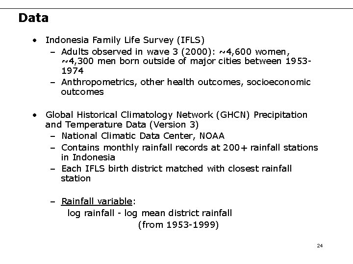
Data • Indonesia Family Life Survey (IFLS) – Adults observed in wave 3 (2000): ~4, 600 women, ~4, 300 men born outside of major cities between 19531974 – Anthropometrics, other health outcomes, socioeconomic outcomes • Global Historical Climatology Network (GHCN) Precipitation and Temperature Data (Version 3) – National Climatic Data Center, NOAA – Contains monthly rainfall records at 200+ rainfall stations in Indonesia – Each IFLS birth district matched with closest rainfall station – Rainfall variable: log rainfall - log mean district rainfall (from 1953 -1999) 24

Early-life rainfall and adult health 25

Early-life rainfall and other outcomes 26

Nonparametric estimates 27

Nonparametric estimates 28

Effect of rainfall before and after birthyear 29

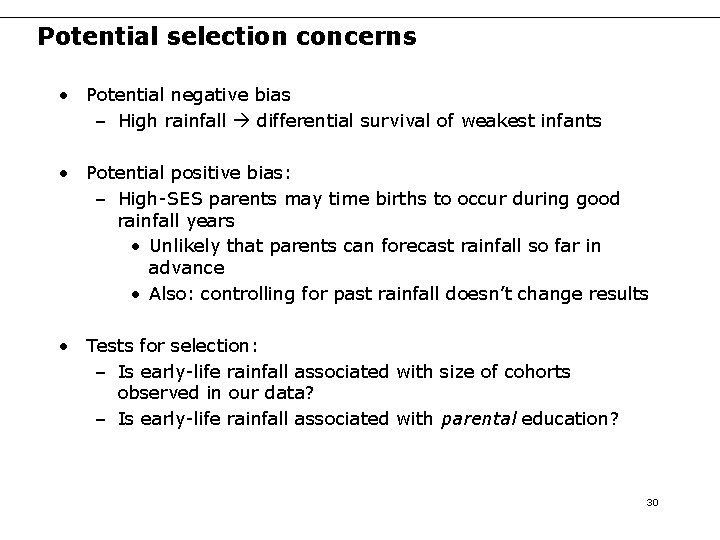
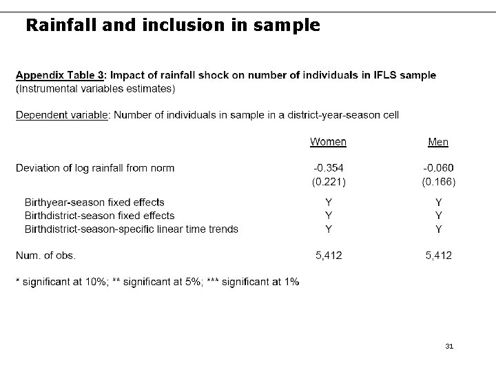
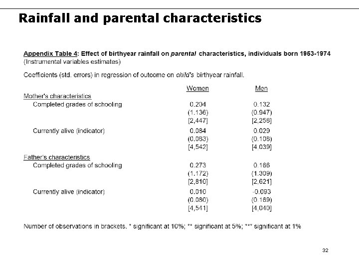
Potential selection concerns • Potential negative bias – High rainfall differential survival of weakest infants • Potential positive bias: – High-SES parents may time births to occur during good rainfall years • Unlikely that parents can forecast rainfall so far in advance • Also: controlling for past rainfall doesn’t change results • Tests for selection: – Is early-life rainfall associated with size of cohorts observed in our data? – Is early-life rainfall associated with parental education? 30

Rainfall and inclusion in sample 31

Rainfall and parental characteristics 32

Pathways to adult SES 33

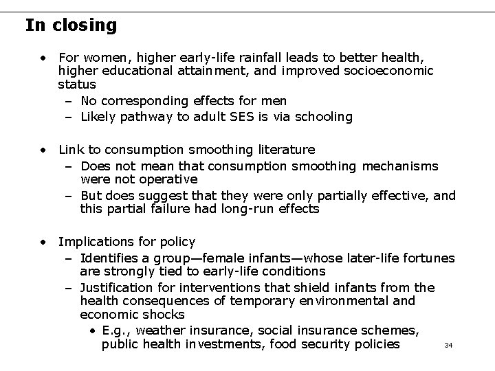
In closing • For women, higher early-life rainfall leads to better health, higher educational attainment, and improved socioeconomic status – No corresponding effects for men – Likely pathway to adult SES is via schooling • Link to consumption smoothing literature – Does not mean that consumption smoothing mechanisms were not operative – But does suggest that they were only partially effective, and this partial failure had long-run effects • Implications for policy – Identifies a group—female infants—whose later-life fortunes are strongly tied to early-life conditions – Justification for interventions that shield infants from the health consequences of temporary environmental and economic shocks • E. g. , weather insurance, social insurance schemes, 34 public health investments, food security policies

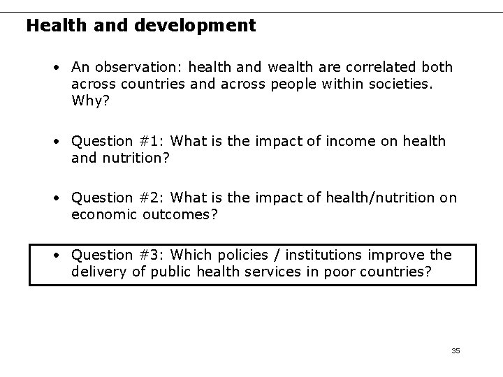
Health and development • An observation: health and wealth are correlated both across countries and across people within societies. Why? • Question #1: What is the impact of income on health and nutrition? • Question #2: What is the impact of health/nutrition on economic outcomes? • Question #3: Which policies / institutions improve the delivery of public health services in poor countries? 35

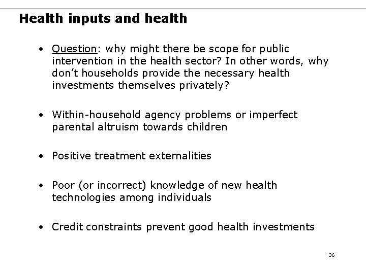
Health inputs and health • Question: why might there be scope for public intervention in the health sector? In other words, why don’t households provide the necessary health investments themselves privately? • Within-household agency problems or imperfect parental altruism towards children • Positive treatment externalities • Poor (or incorrect) knowledge of new health technologies among individuals • Credit constraints prevent good health investments 36

Kremer and Miguel (2004) • Worm infections (e. g. , hookworm, whipworm, roundworm, schistosomiasis) are among the world’s most common infections • Paper studies school-based deworming treatment – In sample of rural Kenyan school children, over 90% were infected at baseline. Between one third and one half had “serious” infections • Worms pass larvae out through human fecal matter, infecting others – Treatment generates a positive externality by reducing this transmission to others 37

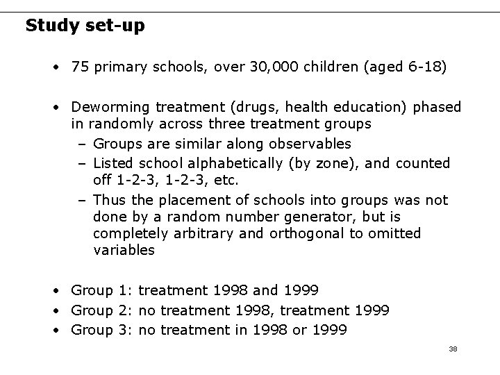
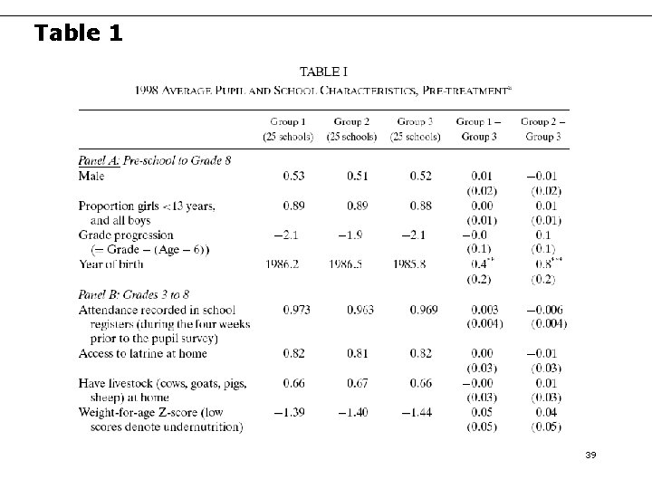
Study set-up • 75 primary schools, over 30, 000 children (aged 6 -18) • Deworming treatment (drugs, health education) phased in randomly across three treatment groups – Groups are similar along observables – Listed school alphabetically (by zone), and counted off 1 -2 -3, etc. – Thus the placement of schools into groups was not done by a random number generator, but is completely arbitrary and orthogonal to omitted variables • Group 1: treatment 1998 and 1999 • Group 2: no treatment 1998, treatment 1999 • Group 3: no treatment in 1998 or 1999 38

Table 1 39

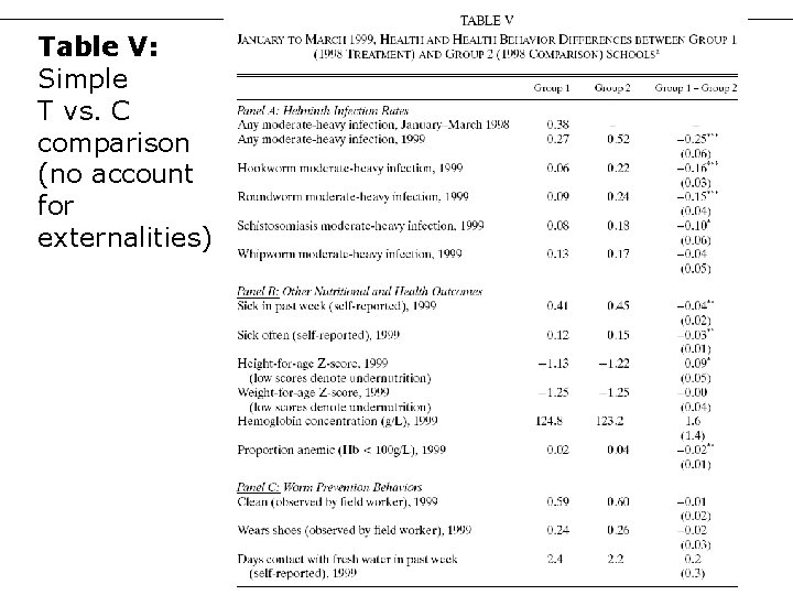
Table V: Simple T vs. C comparison (no account for externalities) 40

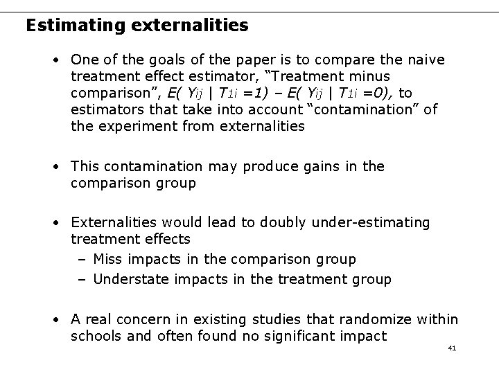
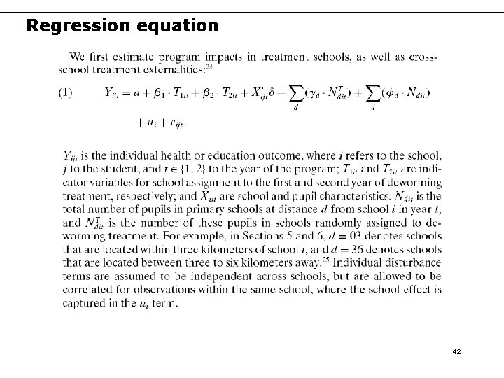
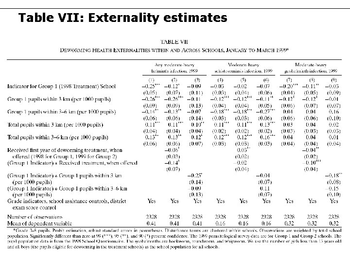
Estimating externalities • One of the goals of the paper is to compare the naive treatment effect estimator, “Treatment minus comparison”, E( Yij | T 1 i =1) – E( Yij | T 1 i =0), to estimators that take into account “contamination” of the experiment from externalities • This contamination may produce gains in the comparison group • Externalities would lead to doubly under-estimating treatment effects – Miss impacts in the comparison group – Understate impacts in the treatment group • A real concern in existing studies that randomize within schools and often found no significant impact 41

Regression equation 42

Table VII: Externality estimates 43

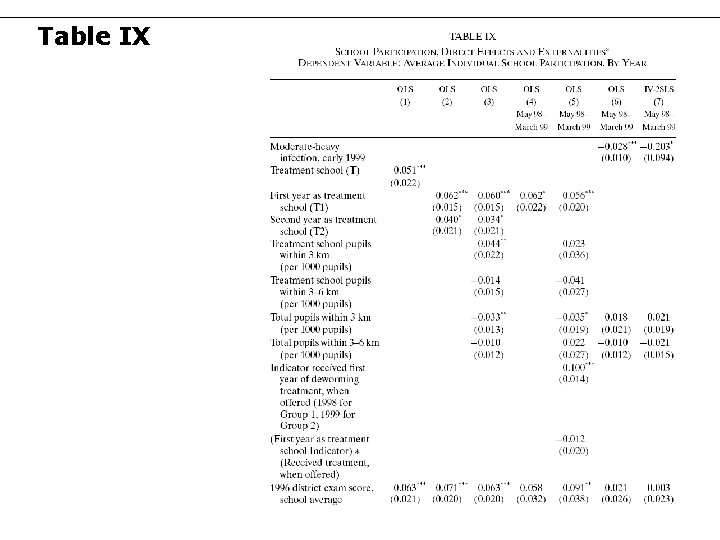
Table IX 44

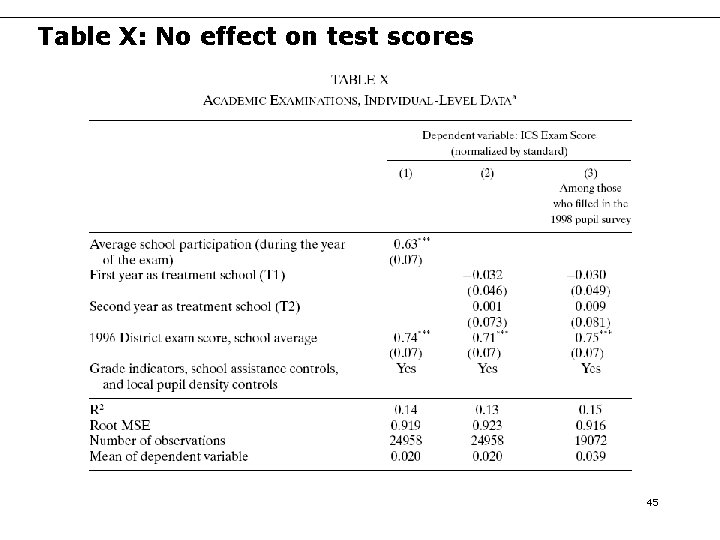
Table X: No effect on test scores 45