HAWKES LEARNING SYSTEMS math courseware specialists Copyright 2008

HAWKES LEARNING SYSTEMS math courseware specialists Copyright © 2008 by Hawkes Learning Systems/Quant Systems, Inc. All rights reserved. Section 2. 1 Frequency Distributions

HAWKES LEARNING SYSTEMS math courseware specialists Graphical Descriptions of Data 2. 1 Frequency Distributions Organizing Data: • Ordered array – an ordered list of the data from largest to smallest or vice versa. Ex. 1 2 2 2 4 5 5 6 • Distribution – displays data values that occur and how often they occur. It can be a chart or a table. 1 1, 2 3, 4 1, 5 2, 6 1 • Frequency Distribution – table that divides data into groups, called classes, and shows how many data values occur in each group. (1 -2 4) • Frequency, f – number of data values in a class. (4)

HAWKES LEARNING SYSTEMS math courseware specialists Graphical Descriptions of Data 2. 1 Frequency Distributions Creating frequency tables: 1. Decide on the number of classes • Between 5 and 20 2. Choose an appropriate class width • 3. Find the class limits • Start with the lowest value and add the class width to get the next class limit. (1 -2, 3 -4, etc) 4. Determine the frequency of each class • Count the number of data values in each class. (1 -2 4)

HAWKES LEARNING SYSTEMS math courseware specialists Graphical Descriptions of Data 2. 1 Frequency Distributions Other characteristics can be calculated once the basic frequency table has been constructed: 1. Classes boundaries • 2. Split the difference in the gap between the upper limit of one class and the lower limit of the next class. (1 -2 0. 5 – 2. 5) Midpoints = 2+1 = 1. 5 2 3. Relative Frequency = 4. 4 8 = 0. 5 (50%) Cumulative Frequency • The sum of the frequency for a given class and all previous classes.

HAWKES LEARNING SYSTEMS math courseware specialists Graphical Descriptions of Data 2. 1 Frequency Distributions Create a frequency distribution using 5 classes: Quiz Grades 9 3 5 4 7 8 10 8 6 7 4 5 2 7 8 10 7 9 10 1 8 6 10 9 8 Solution – First place the data in an ordered array: Quiz Grades – Ordered Array 1 2 3 4 4 5 5 6 6 7 7 8 8 8 9 9 9 10 10

HAWKES LEARNING SYSTEMS math courseware specialists Graphical Descriptions of Data 2. 1 Frequency Distributions Solution – continued: Since we have the smallest and largest values, we can find the class width. Round 1. 8 up to a sensible value, 2. Next begin building the class limits with the smallest data value in the set.

HAWKES LEARNING SYSTEMS math courseware specialists Graphical Descriptions of Data 2. 1 Frequency Distributions The frequency distribution: Quiz Grades Class f Class Boundaries Midpoint Relative Frequency Cumulative Frequency 1– 2 2 0. 5 – 2. 5 1. 5 2 3– 4 3 2. 5 – 4. 5 3. 5 5 5– 6 4 4. 5 – 6. 5 5. 5 9 7– 8 9 6. 5 – 8. 5 7. 5 18 9 – 10 7 8. 5 – 10. 5 9. 5 25 1 2 3 4 4 5 5 6 6 7 7 8 8 8 9 9 9 10 10

HAWKES LEARNING SYSTEMS math courseware specialists Graphical Descriptions of Data 2. 1 Frequency Distributions Create a frequency distribution using 6 classes: GPA’s 3. 2 2. 6 2. 9 2. 0 3. 1 3. 5 1. 8 1. 3 3. 8 3. 0 1. 1 2. 0 2. 5 3. 1 3. 4 Solution – First place the data in an ordered array: GPA’s – Ordered Array 1. 1 1. 3 1. 8 2. 0 2. 5 2. 6 2. 9 3. 0 3. 1 3. 2 3. 4 3. 5 3. 8

HAWKES LEARNING SYSTEMS math courseware specialists Graphical Descriptions of Data 2. 1 Frequency Distributions Solution – continued: Since we have the smallest and largest values, we can find the class width. Round 0. 45 up to a sensible value, 0. 5. Next begin building the class limits with the smallest data value in the set.

HAWKES LEARNING SYSTEMS math courseware specialists Graphical Descriptions of Data 2. 1 Frequency Distributions The frequency distribution: Quiz Grades Class f Class Boundaries Midpoint Relative Frequency Cumulative Frequency 1. 0 – 1. 4 2 0. 95 – 1. 45 1. 2 2 1. 5 – 1. 9 1 1. 45 – 1. 95 1. 7 3 2. 0 – 2. 4 2 1. 95 – 2. 45 2. 2 5 2. 5 – 2. 9 3 2. 45 – 2. 95 2. 7 8 3. 0 – 3. 4 5 2. 95 – 3. 45 3. 2 13 3. 5 – 3. 9 2 3. 45 – 3. 95 3. 7 15 1. 1 1. 3 1. 8 2. 0 2. 5 2. 6 2. 9 3. 0 3. 1 3. 2 3. 4 3. 5 3. 8

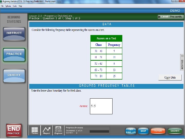
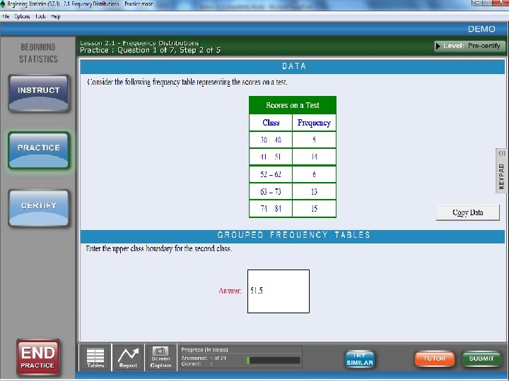
First Class Lower Limit= 29. 5 Upper Limit: =40. 5 Class width = 11 Second Class Lower Limit= 40. 5 Upper Limit: =51. 5 Class width = 11

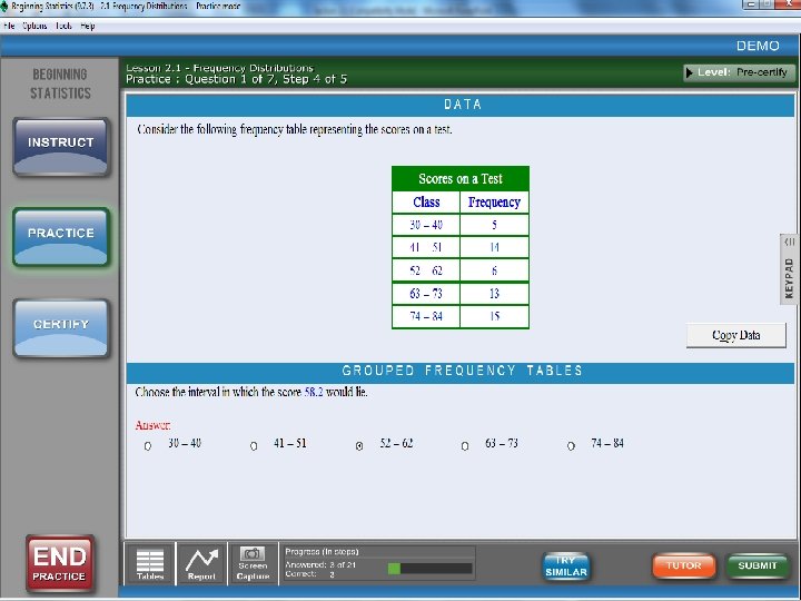
Total = 5 + 14 + 6 + 13 Total = 38

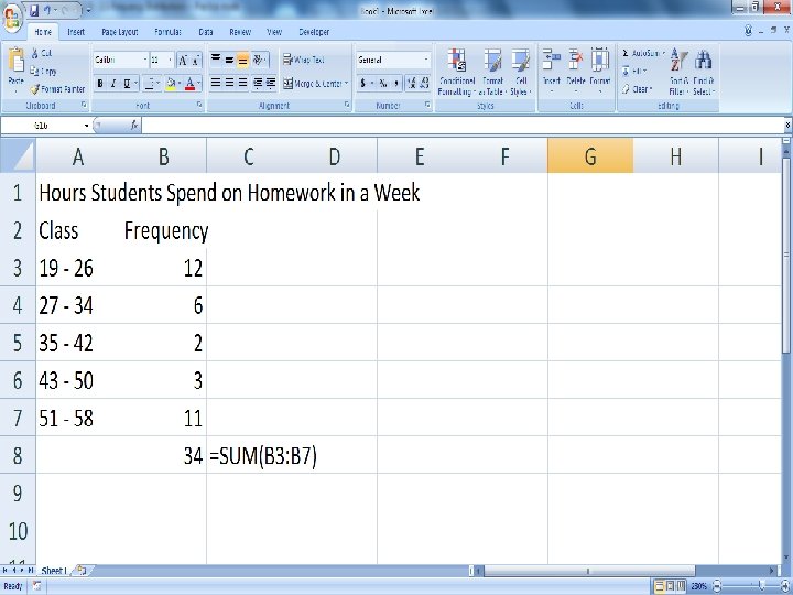
Total = 12 + 6 + 2 + 3 + 11 Total = 34

Mid = 0. 41 + 0. 46 2 Mid = 0. 435