Hard and soft modeling A case study Alexey

Hard and soft modeling. A case study Alexey Pomerantsev Institute of Chemical Physics, Moscow 10. 02. 06 WSC-5 1

Outlines 1. Background 2. Soft modeling 3. Hard modeling 4. Trade-off between hard and soft 10. 02. 06 WSC-5 2

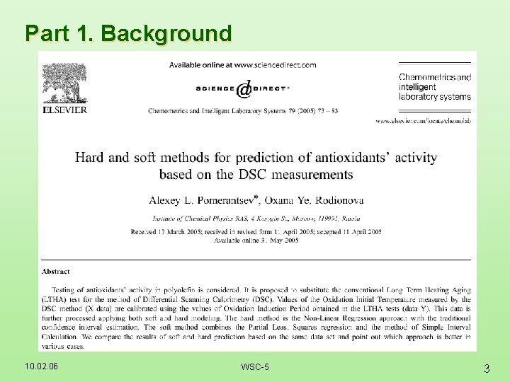
Part 1. Background 10. 02. 06 WSC-5 3

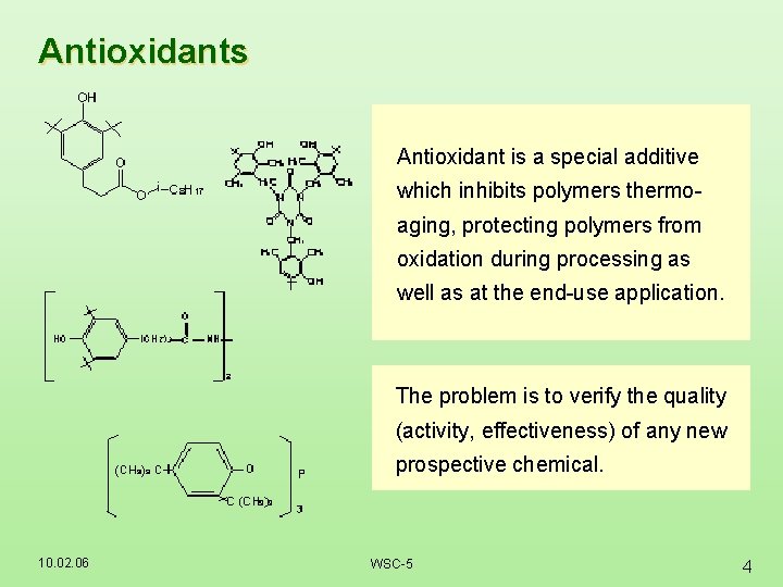
Antioxidants Antioxidant is a special additive which inhibits polymers thermoaging, protecting polymers from oxidation during processing as well as at the end-use application. The problem is to verify the quality (activity, effectiveness) of any new prospective chemical. 10. 02. 06 WSC-5 4

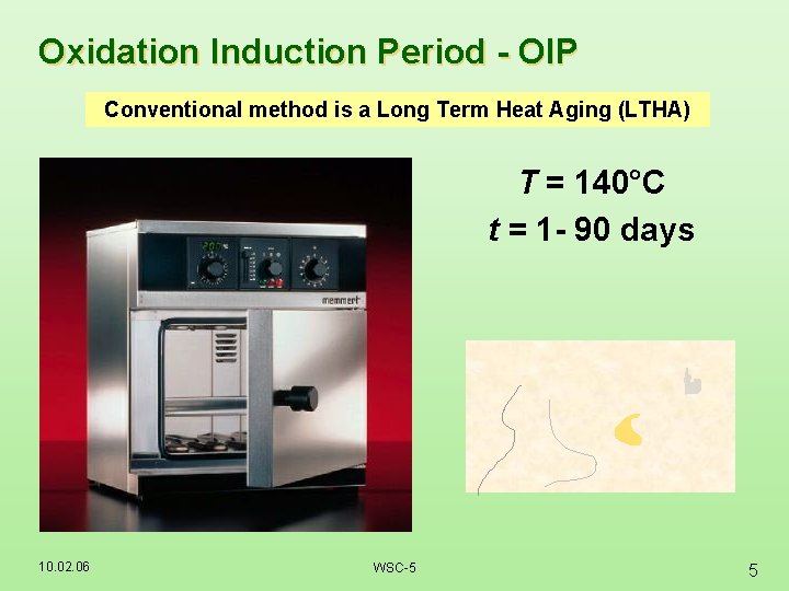
Oxidation Induction Period - OIP Conventional method is a Long Term Heat Aging (LTHA) T = 140°C t = 1 - 90 days 10. 02. 06 WSC-5 5

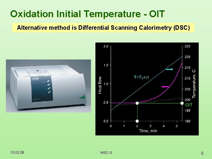
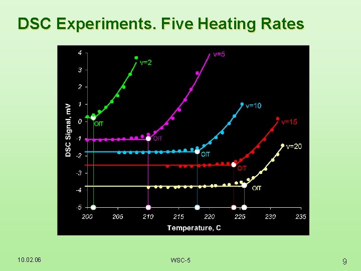
Oxidation Initial Temperature - OIT Alternative method is Differential Scanning Calorimetry (DSC) 10. 02. 06 WSC-5 6

Two Goals approaches trade-off Fast Soft/hard method for the antioxidants testing 1$ 10. 02. 06 WSC-5 7

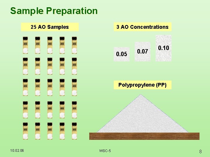
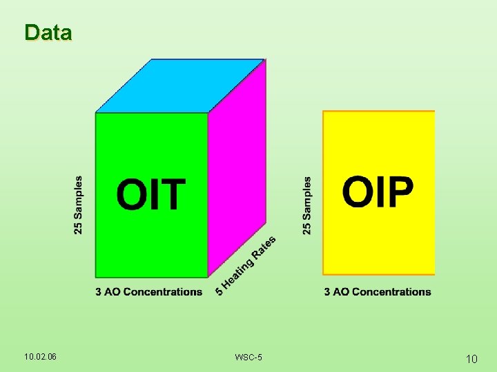
Sample Preparation 3 AO Concentrations 25 AO Samples 0. 05 0. 07 0. 10 Polypropylene (PP) 10. 02. 06 WSC-5 8

DSC Experiments. Five Heating Rates 10. 02. 06 WSC-5 9

Data 10. 02. 06 WSC-5 10

Part 2. Soft Modeling 10. 02. 06 WSC-5 11

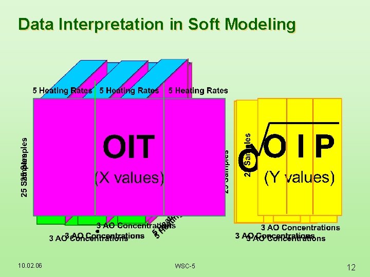
Data Interpretation in Soft Modeling 10. 02. 06 WSC-5 12

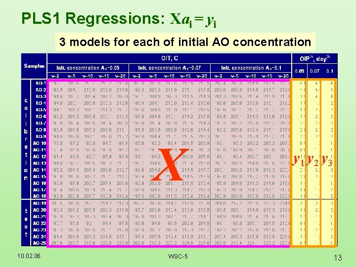
PLS 1 Regressions: Xai = yi 3 models for each of initial AO concentration X 10. 02. 06 WSC-5 y 1 y 2 y 3 13

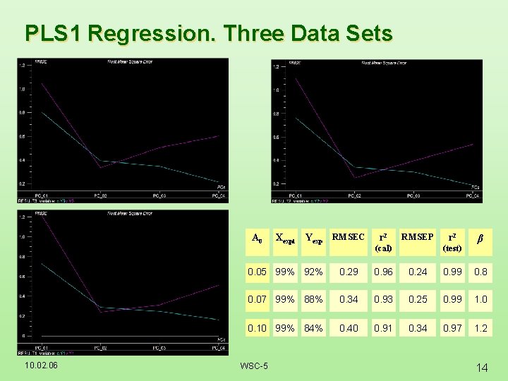
PLS 1 Regression. Three Data Sets A 0 10. 02. 06 Xexpl Yexp RMSEC r 2 RMSEP (cal) r 2 (test) β 0. 05 99% 92% 0. 29 0. 96 0. 24 0. 99 0. 8 0. 07 99% 88% 0. 34 0. 93 0. 25 0. 99 1. 0 0. 10 99% 84% 0. 40 0. 91 0. 34 0. 97 1. 2 WSC-5 14

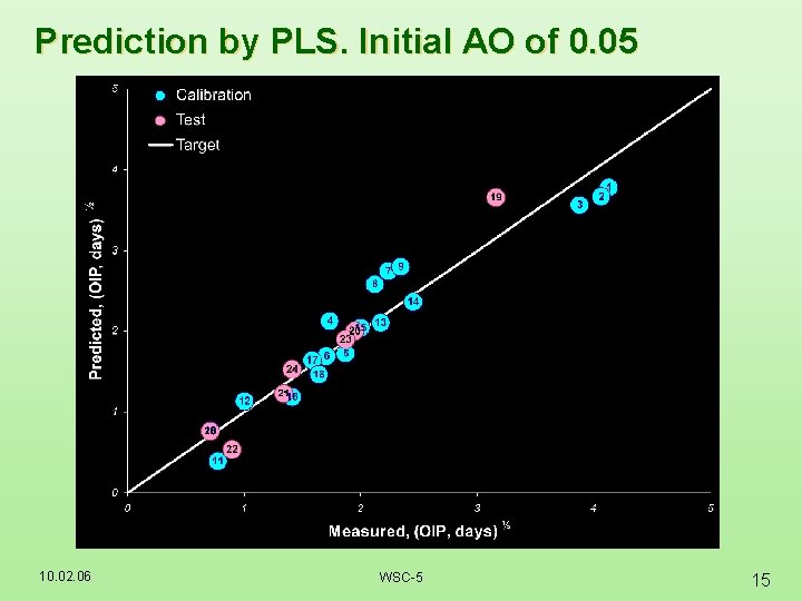
Prediction by PLS. Initial AO of 0. 05 10. 02. 06 WSC-5 15

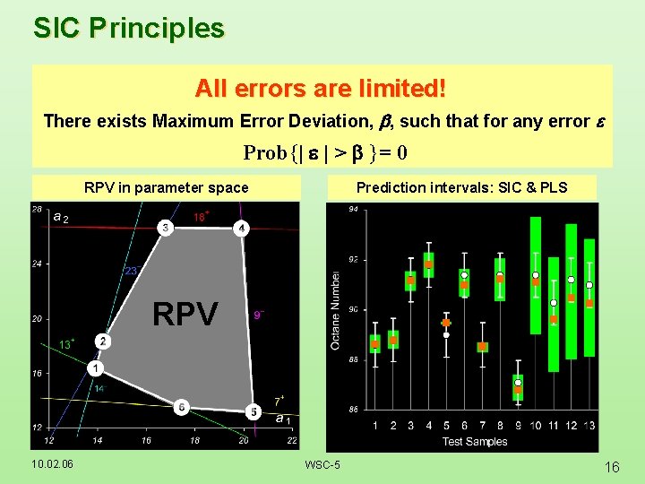
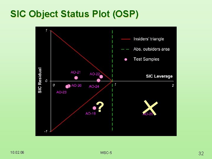
SIC Principles All errors are limited! There exists Maximum Error Deviation, b, such that for any error e Prob{| e | > b }= 0 Prediction intervals: SIC & PLS RPV in parameter space RPV 10. 02. 06 WSC-5 16

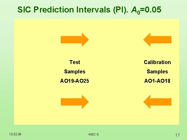
SIC Prediction Intervals (PI). A 0=0. 05 10. 02. 06 Test Calibration Samples AO 19 -AO 25 AO 1 -AO 18 WSC-5 17

Part 3. Hard Modeling 10. 02. 06 WSC-5 18

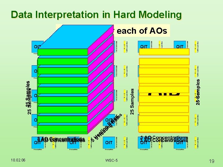
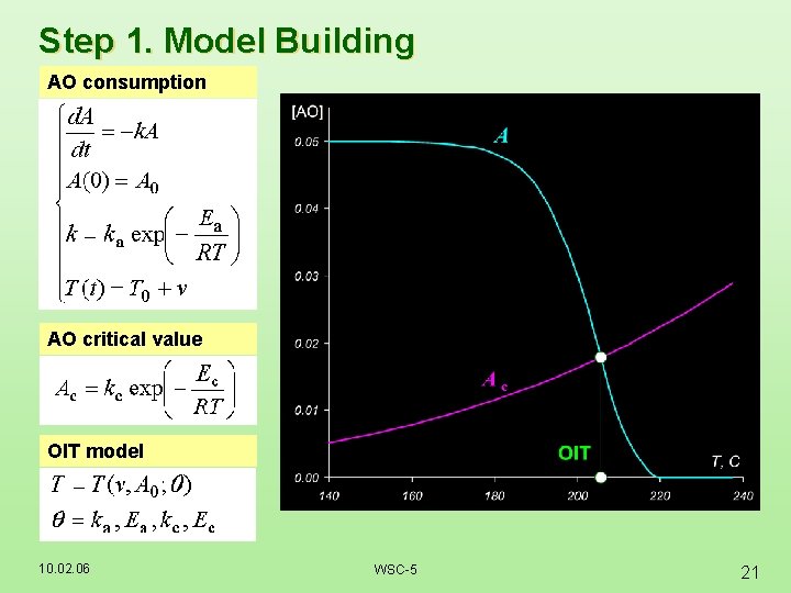
Data Interpretation in Hard Modeling 25 models for each of AOs 10. 02. 06 WSC-5 19

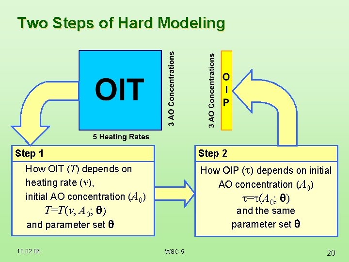
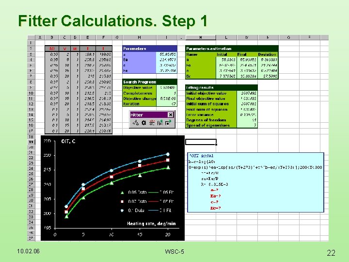
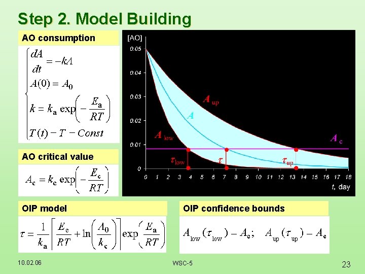
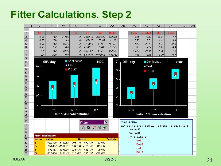
Two Steps of Hard Modeling Step 1 Step 2 How OIP (t) depends on initial AO concentration (A 0) How OIT (T) depends on heating rate (v), initial AO concentration (A 0) t=t(A 0; ) T=T(v, A 0; ) and the same parameter set and parameter set 10. 02. 06 WSC-5 20

Step 1. Model Building AO consumption AO critical value OIT model 10. 02. 06 WSC-5 21

Fitter Calculations. Step 1 10. 02. 06 WSC-5 22

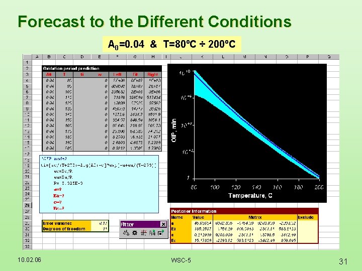
Step 2. Model Building AO consumption AO critical value OIP model 10. 02. 06 OIP confidence bounds WSC-5 23

Fitter Calculations. Step 2 10. 02. 06 WSC-5 24

Part 4. Trade-off between hard and soft 10. 02. 06 WSC-5 25

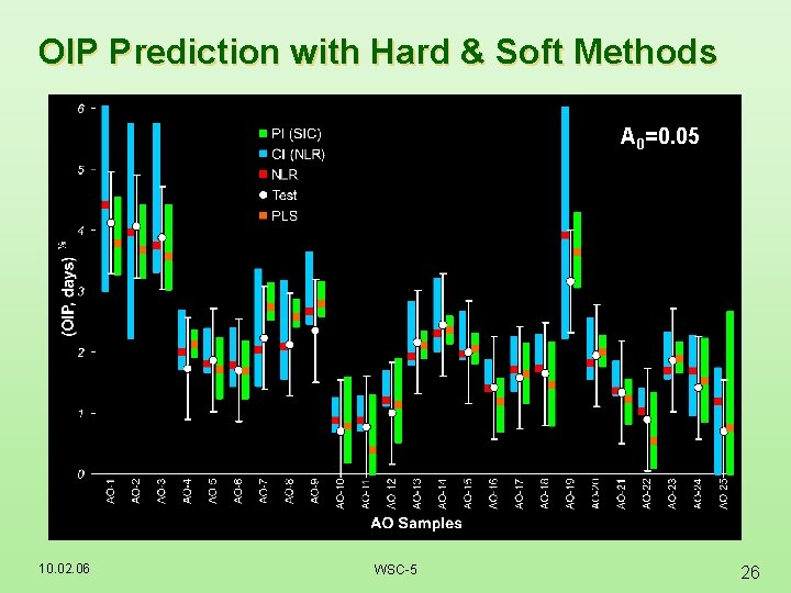
OIP Prediction with Hard & Soft Methods A 0=0. 05 10. 02. 06 WSC-5 26

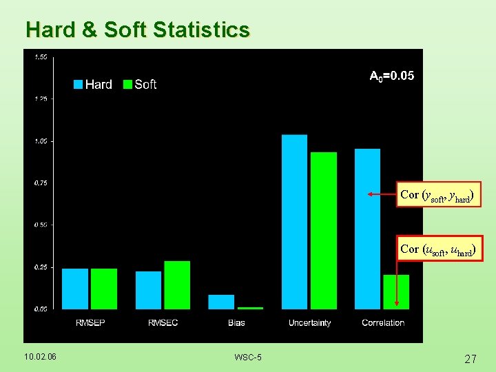
Hard & Soft Statistics Cor (ysoft, yhard) Cor (usoft, uhard) 10. 02. 06 WSC-5 27

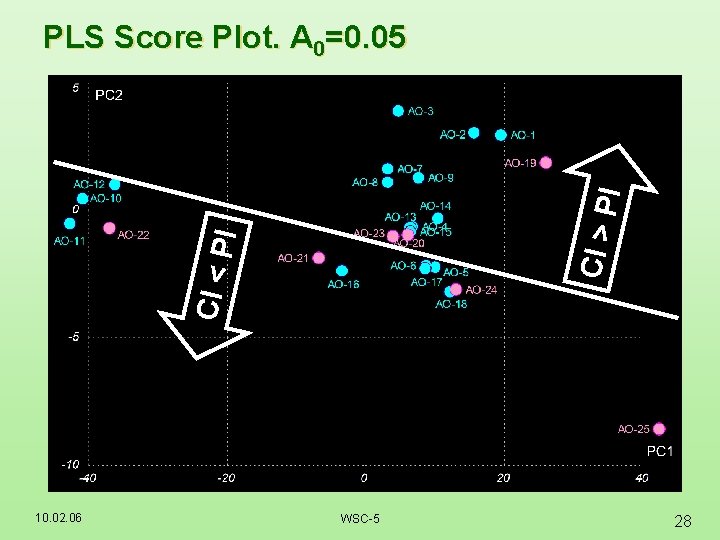
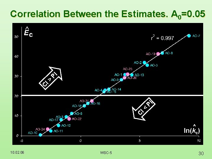
CI < P I CI > P I PLS Score Plot. A 0=0. 05 10. 02. 06 WSC-5 28

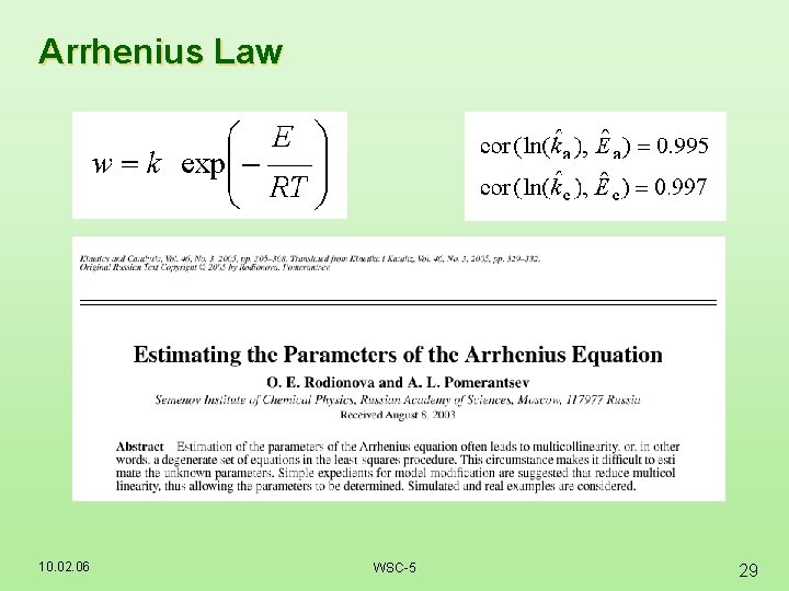
Arrhenius Law 10. 02. 06 WSC-5 29

C I< PI C I> PI Correlation Between the Estimates. A 0=0. 05 ^ ln(kc) 10. 02. 06 WSC-5 30

Forecast to the Different Conditions A 0=0. 04 & T=80ºC ÷ 200ºC 10. 02. 06 WSC-5 31

SIC Object Status Plot (OSP) ? 10. 02. 06 WSC-5 32

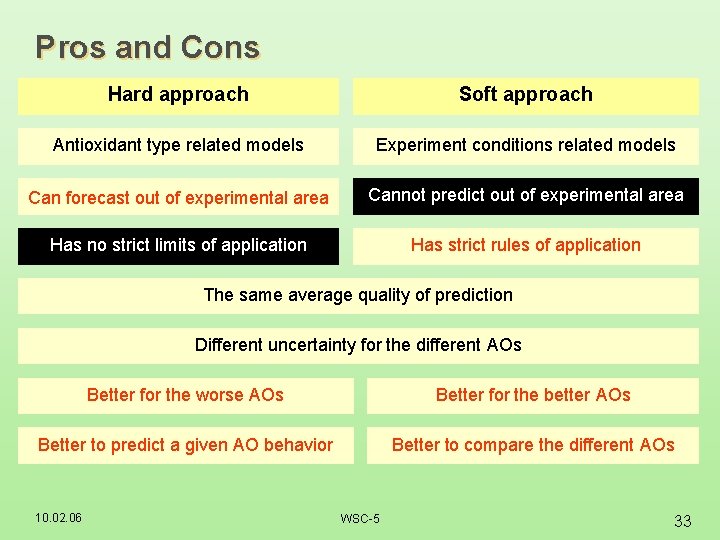
Pros and Cons Hard approach Soft approach Antioxidant type related models Experiment conditions related models Can forecast out of experimental area Cannot predict out of experimental area Has no strict limits of application Has strict rules of application The same average quality of prediction Different uncertainty for the different AOs Better for the worse AOs Better for the better AOs Better to predict a given AO behavior Better to compare the different AOs 10. 02. 06 WSC-5 33

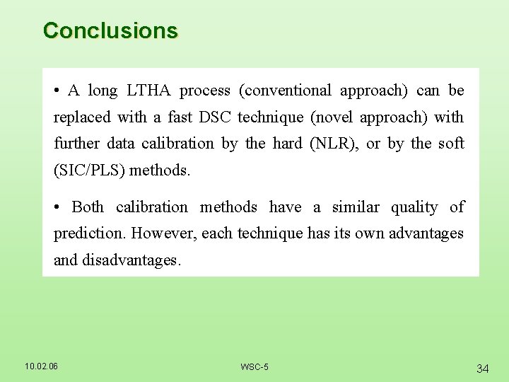
Conclusions • A long LTHA process (conventional approach) can be replaced with a fast DSC technique (novel approach) with further data calibration by the hard (NLR), or by the soft (SIC/PLS) methods. • Both calibration methods have a similar quality of prediction. However, each technique has its own advantages and disadvantages. 10. 02. 06 WSC-5 34