Haplotype assembly Humans are diploid Humans have two

Haplotype assembly

Humans are diploid • Humans have two copies of each chromosome – • Inherited from mother and father. Genotyping technologies do not maintain the phase

Humans are diploid • Genotyping technologies do not maintain the phase

Haplotype phasing using populations • Recall that proximal SNPs are in LD. – – • Few haplotypes must be observed Ex: T|G…G|C is the best phasing of the 1 st two columns This phasing is most reliable for short regions – LD decays at 10 kb

Family based genotyping • If: child is heterozygous, and a parent is homozygous, we know which allele comes from which parent. – – • Location 1: A from mother, T from father Location 2: C from father, G from mother Child haplotypes (TC, AG) Father A/T----C/C Mother A/A----C/G A/T----C/G Child

Sequence based haplotype assembly

Personalized genomics

Haplotype assembly AGAG----CTT------AGT-----A--T ---G------GG---TC------TAG-----AT-AT----GCA------ATG-----TGA ----T---G AGAGCTAGCATGA CTTTTGGTTCGCG • • The fragments are alligned to the unphased reference Uninformative fragments and columns are removed Tri-allelic SNP columns are removed. Relabel the two alleles using 0/1

Haplotype assembly AGAGCTAGCATGA CTTTTGGTTCGCG AGAG----CTT------AGT-----A--T ---G------GG---TC------TAG-----AT-AT----GCA------ATG-----TGA ----T---G • AGAGCTAGCATGA CTTTTGGTTCGCG 0000 ----111 ------001 -----0 --0 ---0 ------10 ------000 -----01 -00 --------000 ----------000 ----1 ---1 Goal: Reconstruct the phased binary string, and its complement, given substrings
")
A Combinatorial problem 0000100 1111011 • Consider a binary string, (and its complement)

• ng 0000 111 001 0 --0 1 ------10 11 000 00 -00 010 100 1 --11 0000100 1111011 stri The string is revealed to us only through a collection of substrings of the string, and its complement. Given the substrings, can the string be reconstructed? sub • s Sampling from the string, and its complement

• • • ng 0000 111 001 0 --0 0 ------10 10 000 01 -00 000 000 1 --11 0000100 1111011 stri • The error free reconstruction is unique. The problem becomes much harder if some of the substrings have errors (do not match the consensus) Define MEC: Minimum # calls that need to be corrected for a match MEC reconstruction: Find the string that minimizes the MEC error. MEC reconstruction is NP-hard even when all fragments have length 2! sub • s Inference in the presence of errors

A simple greedy approach • Greedily select a fragment that extends the current haplotype 0000 ----111 ------001 -----0 --0 ---0 ------10 ------000 -----01 -00 --------000 ----------000 ----1 ---1 0000100 1111011

Extending greedy • • Some fragments will not match without error. These are ‘assigned & corrected’ greedily 0000 ----111 ------001 -----0 --0 ---0 ------10 ------000 -----01 -00 --------000 ----------000 ----1 ---1 0000100 1111011

Greedy haplotype assembly • • • A Greedy scheme such as this was employed for JCV’s genome. MEC: The minimum number of base-calls that need to be flipped for an error free assignment. Goal: reconstruct a haplotype that minimizes MEC 0000 ----111 ------001 -----0 --0 ---0 ------10 ------000 ----- - - 0 1 - 0 0 X- -------000 ----------000 ----1 ---1 0000100 1111011 X X X

Modifying the haplotypes • • The Greedy approach often leads to suboptimal solutions A local flipping of the current haplotype might improve the MEC 0000 ----111 ------001 -----0 --0 ---0 ------10 ------000 ----- - - 0 1 - 0 0 X- -X -------000 ----------000 ----1 ---1 000010000 111101111 X X X

Haplotype to Haplotype • • The haplotype change also involves a reassignment of fragments. Here, the MEC error reduced to 2. This suggests a generic strategy Start with a haplotype, and move to a new one if it can improve the MEC 0000 ----111 ------001 -----0 --0 ---0 ------10 ------000 ----- - - 0 1 - 0 0 - -X -------000 ----------000 ----1 ---1 000010000 111101111 X

A likelihood based approach

A probabilistic formulation Error probability q • We can compute the likelihood of X, given H, q Haplotype H H=(h, h) h: 0 0 1 0 0 0 0 h: 1 1 0 1 1 1 1 • • The goal is to either compute H that maximizes likelihood, OR To sample H from Pr(X|H, q) X 1: 0 0 - - - X 2: X 3: Xn: Fragment matrix X

MCMC sampling of H H H’

An MCMC formulation • A simple neighborhood is defined by flipping one column at a time (Ex: col. 11) – Waterman and Churchill 000010000 111101111 S = {11} 0000100 1111011

Flip-update MC • While this ‘flip-update’ markov chain has the right stationary distribution, it does not converge fast.

A difficult example for the flip-update • • • d n columns, each spanned by d fragments. Two haplotypes (H 1, H 2) are equally likely Hard to move from one good haplotype to another n columns

Mixing times for the flip-update MC • • Let p=1 -q. Mixing time bound based on conductance arguments – • • (Jerrum & Sinclair’ 92) Similar empirical results for hitting time. Even modest values of n, d are problematic. n=20

A simple modification • • • If we modify the neighborhood to include the first n/2 columns… Thm: the mixing time of the Markov Chain is O(n 6), independent of d. Proof uses: – Canonical Paths

A new markov chain

Choosing the neighborhood • The theoretical analysis on examples tells us: – • Choice of neighborhood (subsets of columns that are flipped) is important. Unfortunately, it is not easy to predict what the correct neighborhood should be for an arbitrary example
 is an")
Read-haplotype consistency graph • • Each column is a node. (x, y) is an edge if there is a fragment ‘touching’ columns x and y

Weighting R-H graph edges

Cuts

Negative cuts are good cuts

A combinatorial scheme

Example

First Cut

Graph update

Second cut
")
Hapcut versus sampling • • The Hapcut algorithm allows us (in a heuristic sense) to escape a current local minimum. It can be modified to sample from the Haplotypes, instead of a single haplotype output.

HASH

Haplotype assembly for Huref • • 1. 856 M variants used for haplotype assembly of huref (using an earlier version of the algorithm described here) Chr 22 stats – – – 25 K variant sites, 53 K ‘useful’ rows ~7 variant per fragment 609 disjoint haplotypes (largest contains 1008 variants) N 50 haplotype length=350 Kb (50% of the variant sites lie in haplotypes 350 kb or greater) Paired end sequencing is critical.

Performance on Huref Greedy Hapcut HASH • • • HASH/Hapcut have nearly identical performances HASH is slower but allows for sampling of multiple haplotypes Both offer >20% improvement over the naïve method

Switch error in reconstruction

Simulating errors Errors were simulated on Huref sequences • Switch error in reconstruction is low, and decreases with increased depth • The computed MEC error tracks simulated errors •

Measuring switch errors • A switch w. r. t hapmap phasing is illustrative of either low LD, or HASH error
")
Comparison against Hapmap • • HASH mismatch rate is low (0. 008 -0. 03) Adjusted rate – • • (0. 008 -0. 011) Hapmap error rate is 0. 005 (CEU) to 0. 02 (YRI) even with trios Without trios, error is 0. 05

Did we cheat? is Read Length Important? • • Haplotyping results would be very poor with Next gen sequencing If 250, 000 long reads were available, could we solve the assembly problem? 200, 000 5000 150, 000 4000 AN 50 Adjusted N 50 6000 100, 000 3000 2000 1000 50, 000 0 0 • 1000 2000 3000 4000 5000 6000 Read Length 7000 8000 1000 Read Length 9000 10000 Conclusion: Read-length helps, but we need very long reads to achieve reasonable N 50 2000

The two challenges of Haplotype assembly • • Accuracy of haplotypes solved using computation (HASH/Hapcut) Length of haplotypes: – – – Described by the number of nodes in the graph Primarily a technology issue. Sanger sequencing: • – Next Gen sequencing: • – long haplotypes, prohibitively expensive Affordable, short haplotypes Single molecule sequencing • • ‘longer’ reads, but, … Ability to switch sequencing ON/OFF in a strobe mode

Should paired end gap be varied? • Fix: Read Length, Coverage, Max Insert Size to keep cost constant Varying insert improves haplotype length Varying Advance Lengths 80000 70000 60000 50000 AN 50 • 40000 30000 20000 10000 0 0 20 40 60 80 % of advance lengths = 9000 bp (100 -x)% of advance lengths = 3000 bp 100 120

The two challenges of Haplotype assembly • • Accuracy of haplotypes solved using computation (HASH/Hapcut) Length of haplotypes: – – – Described by the number of nodes in the graph Primarily a technology issue. Sanger sequencing: • – Next Gen sequencing: • – long haplotypes, prohibitively expensive Affordable, short haplotypes Single molecule sequencing • • ‘longer’ reads, but, … Ability to switch sequencing ON/OFF in a strobe mode
 f(a) on advance")
Varying advance lengths • We need to find a distribution (pdf) f(a) on advance length a that will optimize AN 50 Q: Compute the shape that maximizes AN 50 f(a) Advance length a

Beta Distribution • • Optimization over different shapes is difficult. Our solution: Use the beta distribution Pros: Only two parameters Cons: Considers a limited sampling of the space.

Varying Advance Length • Choosing the right distribution of advance lengths • Varying α, β parameters of the β-distribution 160000 Distribution of advance length for a=1. 6 b=0. 5 140000 120000 Distribution of advance length for a=0. 6 b=2. 1 100000 AN 50 80000 60000 40000 20000 0 0. 1 0. 2 0. 3 0. 4 0. 5 0. 6 0. 7 0. 8 0. 9 1 1. 2 1. 3 1. 4 1. 5 1. 6 1. 7 1. 8 1. 9 2 2. 1 2. 2 2. 3 2. 4 2. 5 2. 6 2. 7 2. 8 2. 9 3 Distribution of advance length for a=1 b=1

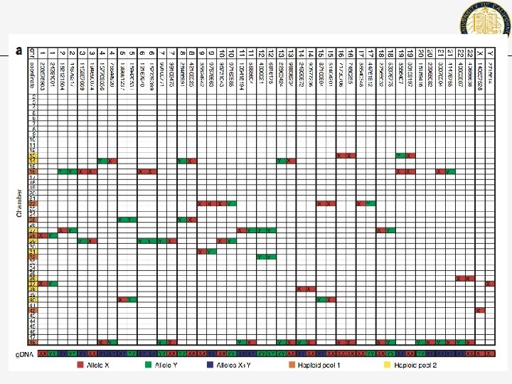
Other technologies for haplotyping • • • Isolate a single cell from suspension Use protease digestion to release all DNA from the cytoplasm (46 chromosomes) Randomly partition chromosomes into 48 chambers Multiple strand displacement amplification of single genomes (This is the tricky part) in each tube Test each tube for heterozygozity Genotype each homozygous tube

Loci Tubes • chr 1 • X • A small PCR based test is used to see which chromosome is in which tube (marked by X) How many marks per locus should we see? We can combine the content of two tubes if they do not contain homologous pairs. Finally, we genotype the remaining pairs/sequence them.
 by considering sources of variation Models")
Topics covered 1. 2. We started (and finished) by considering sources of variation Models of evolution of population under natural assumptions 1. 2. 3. 4. 5. 6. 7. HW/Linkage equlibrium Efficient simulation of populations via coalescent theory Detecting structural variation Detection of regions under selection Association testing Population sub-structure Haplotype phasing
")
Algorithmic diversions 1. 2. 3. 4. 5. 6. Phylogeny reconstruction (perfect phylogeny, distancebased methods) Optimization using (Integer-) Linear programming, simulated annealing and other paradigms. Maximum flows. Greedy algorithms, dynamic programming Stochastic sampling methods (MCMC, Gibbs sampling) Statistical tests for significance Efficient simulation techniques 1. 2. Coalescent for populations, including recombination, selection, etc. Simulating genotype/phenotype associations
 by considering sources of variation Models")
Topics covered 1. 2. We started (and finished) by considering sources of variation Models of evolution of population under natural assumptions 1. 2. 3. 4. 5. 6. 7. 8. HW/Linkage equlibrium Efficient simulation of populations via coalescent theory Detecting structural variation Detection of regions under selection Association testing Population sub-structure Evolution under recombinations/recombination hot-spot detection via counting of recombination events (partially) Haplotype phasing (partially)
")
Algorithmic diversions 1. 2. 3. 4. 5. 6. Phylogeny reconstruction (perfect phylogeny, distancebased methods) Optimization using (Integer-) Linear programming, simulated annealing and other paradigms Greedy algorithms, dynamic programming Stochastic sampling methods (MCMC, Gibbs sampling) Statistical tests for significance Efficient simulation techniques 1. 2. 3. Coalescent for populations Simulating genotype/phenotype associations Pairwise analysis
- Slides: 58