Handout 7 Interaction and Higher Order Terms in

Handout 7: Interaction and Higher. Order Terms in Regression Thomas & Monin Psych 252 2010

Higher-Order Terms

Polynomial Terms: Centering

Notice how if all your values are positive, x and x 2 are collinear.

Uncentered: Standardized:

> rnorm(100, mean=5, sd=2)->x > mean(x) [1] 4. 647137 > sd(x) [1] 2. 114859 > scale(x)->zx > mean(zx) [1] 4. 152277 e-17 > sd(zx) [1] 1 > scale(x, scale=F)->cx > mean(cx) [1] 8. 906938 e-17 > sd(cx) [1] 2. 114859 > cor(cbind(cx, zx, x, x-mean(x))) x 1 1 1 1 > cbind(x, zx, cx, x-mean(x)) x [1, ] 5. 5186121 0. 412072404 0. 871474853 [2, ] 4. 3619941 -0. 134828505 -0. 285143217 [3, ] 8. 2563399 1. 706592911 3. 609202630 [4, ] 10. 7328228 2. 877585140 6. 085685572 [5, ] 5. 7731616 0. 532434822 1. 126024342 [6, ] 3. 4313535 -0. 574877106 -1. 215783770 (…)

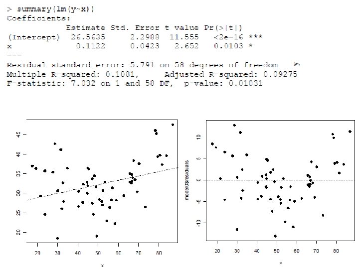
Uncentered: Note the odd negative linear coefficient…

Let’s think about what a quadratic term means: So the slope of X 1 increases with X 1: So b 1 is the slope of X 1 at X 1 = 0:

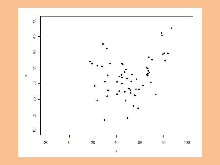
Without centering, the linear coefficient is the tangent at X = 0, which may be meaningless.

Uncentered: Now the negative coefficient makes sense! It is the (tangential) slope when x = 0.

When you center, the linear coefficient is the tangent at the mean of X.

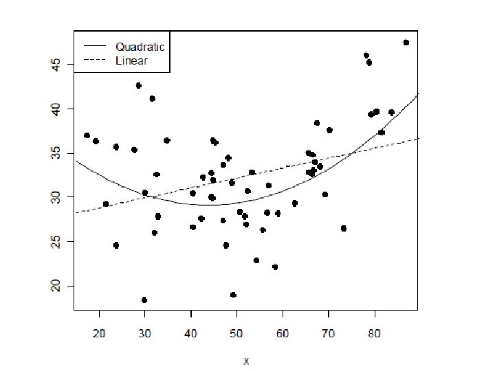
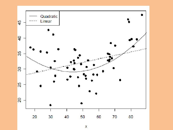
Uncentered: Centered: > summary(lm(y~I(x-mean(x))+I((x-mean(x))^2))) Coefficients: Estimate Std. Error t value Pr(>|t|) (Intercept) 29. 445251 0. 852829 34. 527 < 2 e-16 *** I(x - mean(x)) 0. 103482 0. 035615 2. 906 0. 00521 ** I((x - mean(x))^2) 0. 009230 0. 001845 5. 003 5. 74 e-06 *** --- With centering, the linear coefficient is close to what you obtain with just a linear predictor in the equation. Residual standard error: 4. 87 on 57 degrees of freedom Multiple R-squared: 0. 3802, Adjusted R-squared: 0. 3585 F-statistic: 17. 49 on 2 and 57 DF, p-value: 1. 198 e-06

With centering, the linear coefficient is close to what you obtain with just a linear predictor in the equation.

Centered: Using poly():

Interaction Between a Continuous and a Categorical Variable

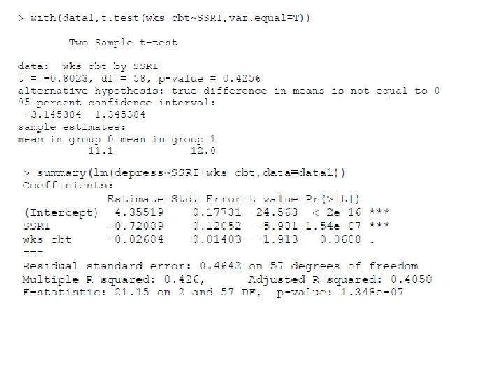
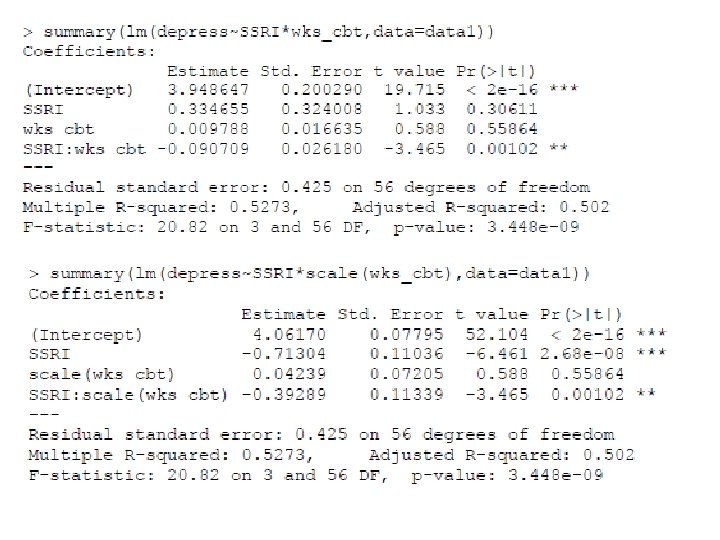
With centering wks_cbt, the coefficients for the interaction and for wks_cbt don’t change… Call: lm(formula = depress ~ SSRI * I(wks_cbt - mean(wks_cbt)), data = data 1) Coefficients: Estimate Std. Error t value Pr(>|t|) (Intercept) 4. 061697 0. 077953 52. 104 < 2 e-16 *** SSRI -0. 713038 0. 110363 -6. 461 2. 68 e-08 *** I(wks_cbt - mean(wks_cbt)) 0. 009788 0. 016635 0. 588 0. 55864 SSRI: I(wks_cbt - mean(wks_cbt)) -0. 090709 0. 026180 -3. 465 0. 00102 ** Residual standard error: 0. 425 on 56 degrees of freedom Multiple R-squared: 0. 5273, Adjusted R-squared: 0. 502 F-statistic: 20. 82 on 3 and 56 DF, p-value: 3. 448 e-09

… but the intercept and the coefficient for SSRI does. Call: lm(formula = depress ~ SSRI * I(wks_cbt - mean(wks_cbt)), data = data 1) Coefficients: Estimate Std. Error t value Pr(>|t|) (Intercept) 4. 061697 0. 077953 52. 104 < 2 e-16 *** SSRI -0. 713038 0. 110363 -6. 461 2. 68 e-08 *** I(wks_cbt - mean(wks_cbt)) 0. 009788 0. 016635 0. 588 0. 55864 SSRI: I(wks_cbt - mean(wks_cbt)) -0. 090709 0. 026180 -3. 465 0. 00102 ** Residual standard error: 0. 425 on 56 degrees of freedom Multiple R-squared: 0. 5273, Adjusted R-squared: 0. 502 F-statistic: 20. 82 on 3 and 56 DF, p-value: 3. 448 e-09

Let’s think about what an interaction term means: So the slope of X 1 increases with X 2: So b 1 is the slope of X 1 at X 2 = 0:

Now I’ve centered wks_cbt…

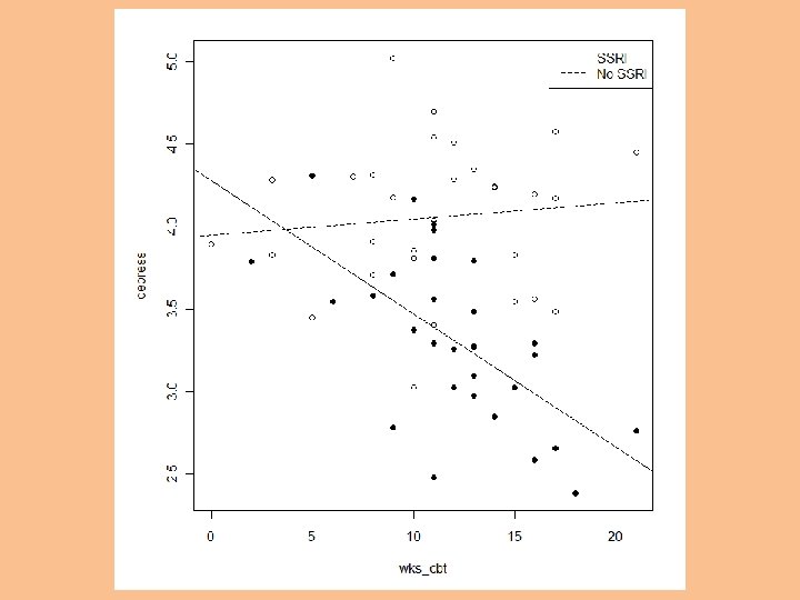
… and the regression lines look the same.

Now we see what the b for SSRI means with or without centering. +. 33 (uncentered) -. 71 (centered)

Call: lm(formula = depress ~ SSRI * I(wks_cbt - mean(wks_cbt)), data = data 1) Coefficients: Estimate Std. Error t value Pr(>|t|) (Intercept) 4. 061697 0. 077953 52. 104 < 2 e-16 *** SSRI -0. 713038 0. 110363 -6. 461 2. 68 e-08 *** I(wks_cbt - mean(wks_cbt)) 0. 009788 0. 016635 0. 588 0. 55864 SSRI: I(wks_cbt - mean(wks_cbt)) -0. 090709 0. 026180 -3. 465 0. 00102 ** Residual standard error: 0. 425 on 56 degrees of freedom Multiple R-squared: 0. 5273, Adjusted R-squared: 0. 502 F-statistic: 20. 82 on 3 and 56 DF, p-value: 3. 448 e-09

> summary(lm(depress~I(wks_cbt-mean(wks_cbt))*SSRI, data=data 1)) Coefficients: Estimate Std. Error t value Pr(>|t|) (Intercept) 4. 061697 0. 077953 52. 104 < 2 e-16 *** I(wks_cbt - mean(wks_cbt)) 0. 009788 0. 016635 0. 588 0. 55864 SSRI -0. 713038 0. 110363 -6. 461 2. 68 e-08 *** I(wks_cbt - mean(wks_cbt)): SSRI -0. 090709 0. 026180 -3. 465 0. 00102 ** Thus “effect coding” of factors is equivalent to centering with equal-size cells. > summary(lm(depress~I(wks_cbt-mean(wks_cbt))*I(SSRI-mean(SSRI)), data=data 1)) Coefficients: Estimate Std. Error (Intercept) 3. 70518 0. 05518 I(wks_cbt - mean(wks_cbt)) -0. 03557 0. 01309 I(SSRI - mean(SSRI)) -0. 71304 0. 11036 I(wks_cbt - mean(wks_cbt)): I(SSRI - mean(SSRI)) (…) -0. 09071 0. 02618 t value Pr(>|t|) 67. 145 < 2 e-16 *** -2. 717 0. 00875 ** -6. 461 2. 68 e-08 *** -3. 465 0. 00102 ** > factor(data 1$SSRI)->data 1$f. SSRI ## Making SSRI a factor > contrasts(data 1$f. SSRI)<-c(-1, 1) ## Effect coding > summary(lm(depress~I(wks_cbt-mean(wks_cbt))*f. SSRI, data=data 1)) Coefficients: Estimate Std. Error t value Pr(>|t|) (Intercept) 3. 70518 0. 05518 67. 145 < 2 e-16 *** I(wks_cbt - mean(wks_cbt)) -0. 03557 0. 01309 -2. 717 0. 00875 ** f. SSRI 1 -0. 35652 0. 05518 -6. 461 2. 68 e-08 *** I(wks_cbt - mean(wks_cbt)): f. SSRI 1 -0. 04535 0. 01309 -3. 465 0. 00102 **

The b 1 slope for wks_cbt when SSRI is effect-coded (equaln) or centered is the “average” slope for b 1 across values of SSRI.

> table(cbt$SSRI) 0 1 30 30 > cbt[-c(50: 60), ]->cbt 2 > table(cbt 2$SSRI) 0 1 19 30 > table(scale(cbt 2$SSRI, scale=F)) -0. 612244897959184 0. 387755102040816 19 30 > contrasts(cbt 2$f. SSRI) [, 1] 0 -1 1 1 With unequal n’s, centering and effect coding depart… but can both be valid, depending on whether you cell sizes are representative. > summary(lm(depress~f. SSRI*scale(wks_cbt, scale=F), data=cbt 2)) # Effect coded Estimate Std. Error t value Pr(>|t|) (Intercept) 3. 66046 0. 06326 57. 866 < 2 e-16 *** f. SSRI 1 -0. 35152 0. 06326 -5. 557 1. 41 e-06 *** scale(wks_cbt, scale = F) -0. 02746 0. 01833 -1. 498 0. 1410 f. SSRI 1: scale(wks_cbt, scale = F) -0. 05346 0. 01833 -2. 917 0. 0055 ** > summary(lm(depress~scale(SSRI, scale=F)*scale(wks_cbt, scale=F), data=cbt 2)) # Centered Coefficients: Estimate Std. Error t value Pr(>|t|) (Intercept) 3. 58155 0. 06164 58. 103 < 2 e-16 *** scale(SSRI, scale = F) -0. 70305 0. 12651 -5. 557 1. 41 e-06 *** scale(wks_cbt, scale = F) -0. 03946 0. 01722 -2. 292 0. 0267 * scale(SSRI, scale = F): scale(wks_cbt, scale = F) -0. 10692 0. 03665 -2. 917 0. 0055 **

Slopes with Centered Predictors With all centered predictors, each first-order coefficient is readily interpretable as: 1. The slope for that predictor at the sample mean of all other variables in the equation. 2. The average slope for that predictor across the range of the other predictors in the equation.

Interaction Between Continuous Variables

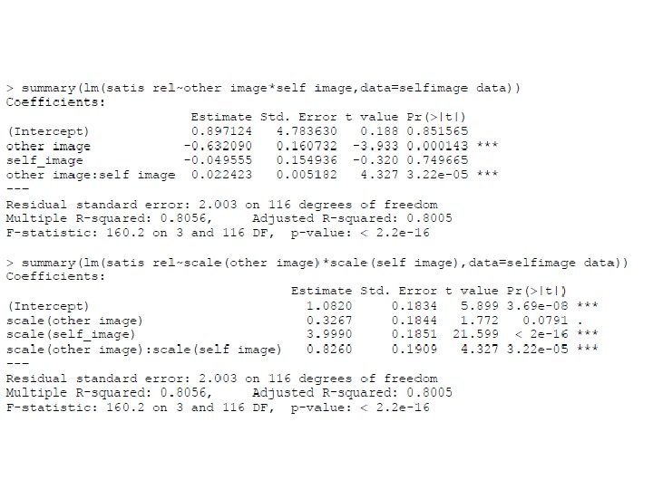
> modelsv<-lm(satis_rel~self_image*other_image, data=selfimage_data) > summary(modelsv) Coefficients: Estimate Std. Error t value Pr(>|t|) (Intercept) 0. 897124 4. 783630 0. 188 0. 851565 self_image -0. 049555 0. 154936 -0. 320 0. 749665 other_image -0. 632090 0. 160732 -3. 933 0. 000143 *** self_image: other_image 0. 022423 0. 005182 4. 327 3. 22 e-05 *** --Residual standard error: 2. 003 on 116 degrees of freedom Multiple R-squared: 0. 8056, Adjusted R-squared: 0. 8005 F-statistic: 160. 2 on 3 and 116 DF, p-value: < 2. 2 e-16 > modelsv_m<-lm(satis_rel~self_image+other_image+ I(self_image*other_image)) > summary(modelsv_m) Coefficients: Estimate Std. Error t value Pr(>|t|) (Intercept) 0. 897124 4. 783630 0. 188 0. 851565 self_image -0. 049555 0. 154936 -0. 320 0. 749665 other_image -0. 632090 0. 160732 -3. 933 0. 000143 *** I(self_image * other_image) 0. 022423 0. 005182 4. 327 3. 22 e-05 *** --Residual standard error: 2. 003 on 116 degrees of freedom Multiple R-squared: 0. 8056, Adjusted R-squared: 0. 8005 F-statistic: 160. 2 on 3 and 116 DF, p-value: < 2. 2 e-16 This is to drive home that an interaction term is literally a product term.

An example of “non-essential multicollinearity” – that variables are correlated with their product, unless centered: self other s_X_o c_self c_other cs_x_co self 1. 00 0. 07 0. 75 1. 00 0. 07 -0. 11 other 0. 07 1. 00 0. 70 0. 07 1. 00 -0. 06 s_X_o 0. 75 0. 70 1. 00 0. 75 0. 70 0. 01 c_self 1. 00 0. 07 0. 75 1. 00 0. 07 -0. 11 c_other 0. 07 1. 00 0. 70 0. 07 1. 00 -0. 06 cs_x_co -0. 11 -0. 06 0. 01 -0. 11 -0. 06 1. 00 If X 1 and X 2 are perfectly symmetrical (notice what happens when the means are zero): What remains after centering is “essential multicollinearity. ” The correlations above are non-null because the variables are not completely symmetrical.

Illustrating non-essential multicollinearity. These two variables are clearly uncorrelated…

… yet their product seems correlated with both.

… unless we center them. Think of projecting the dots on the two “walls” to see why multicollinearity is reduced.

We could also center if we prefer: > > selfimage_data$self_image-mean(selfimage_data$self_image)->c_selfimage_data$other_image-mean(selfimage_data$other_image)->c_other lm(satis_rel~c_self*c_other, data=selfimage_data)->model 1 summary(model 1) Coefficients: (Intercept) c_self c_other c_self: c_other Estimate Std. Error t value Pr(>|t|) 1. 081998 0. 183412 5. 899 3. 69 e-08 0. 622226 0. 028808 21. 599 < 2 e-16 0. 057003 0. 032177 1. 772 0. 0791 0. 022423 0. 005182 4. 327 3. 22 e-05 *** > lm(satis_rel~scale(self)*scale(other), data=selfimage_data)->model 2 > summary(model 2) Coefficients: Estimate Std. Error t value Pr(>|t|) (Intercept) 1. 0820 0. 1834 5. 899 3. 69 e-08 scale(self) 3. 9990 0. 1851 21. 599 < 2 e-16 scale(other) 0. 3267 0. 1844 1. 772 0. 0791 scale(self): scale(other) 0. 8260 0. 1909 4. 327 3. 22 e-05 *** Here I prefer standardizing [scale()] because the units are arbitrary.

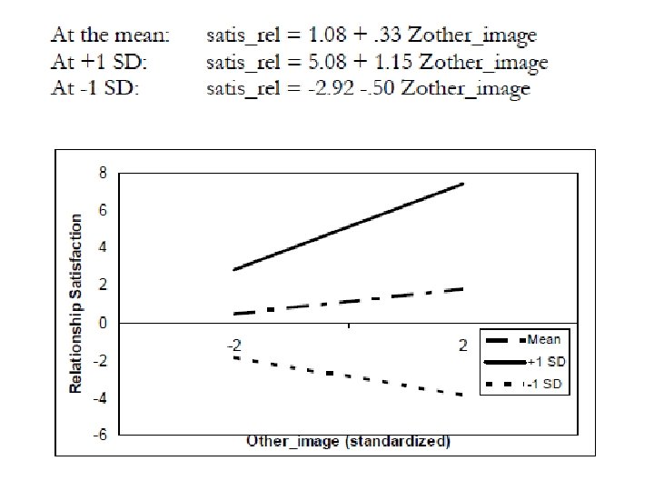
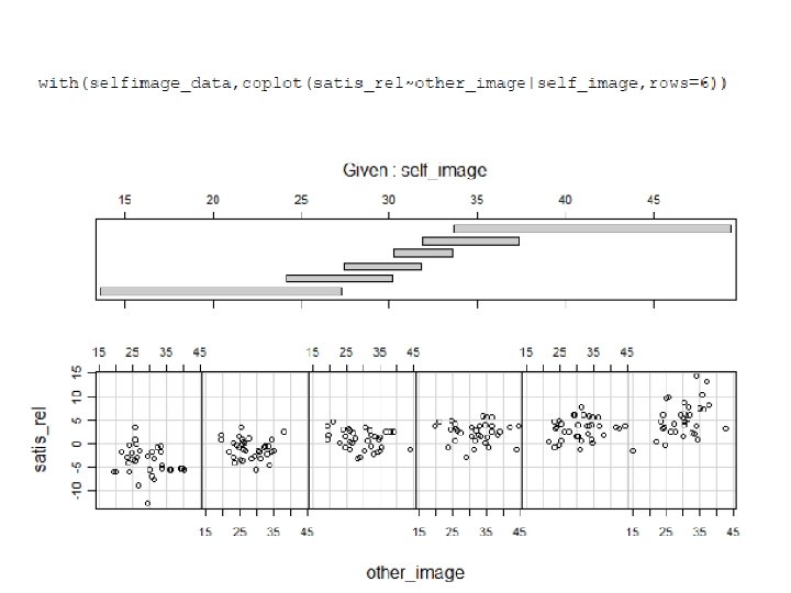
This is to illustrate that the interaction spans the whole space, creating an infinity of different slopes.

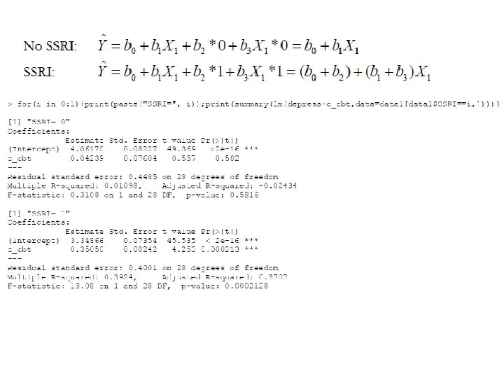
Are these “simple slopes” significant?

Testing Simple Slopes The slope of X 1 at X 2 is: Its standard error is:

First obtain the variance-covariance matrix of the coefficients: > vcov(model 2) (Intercept) scale(self) scale(other) (Intercept) 0. 0336399684 -0. 0002693481 -0. 0001418956 scale(self) -0. 0002693481 0. 0342799579 -0. 0023154183 scale(other) -0. 0001418956 -0. 0023154183 0. 0340130074 scale(self): scale(other) -0. 0026748440 0. 0036694036 0. 0019330832 scale(self): scale(other) -0. 002674844 0. 003669404 0. 001933083 0. 036440137 > vcov(model 2)->m > bm. sesimple<-function(self){sqrt(m[3, 3]+self^2*m[4, 4]+2*self*m[3, 4])} > (model 2$coeff[3]+(0)*model 2$coeff[4])/bm. sesimple(0) scale(other) 1. 771509 > (model 2$coeff[3]+(1)*model 2$coeff[4])/bm. sesimple(1) scale(other) 4. 228297 > (model 2$coeff[3]+(-1)*model 2$coeff[4])/bm. sesimple(-1) scale(other) -1. 934840

bm. tsimple<-function(self) {(model 2$coeff[3]+(self)*model 2$coeff[4])/bm. sesimple(self curve(bm. tsimple, xlim=c(-6, 6), lwd=3) lines(c(0, 0), c(-5, 5)) lines(c(-7, 7), c(0, 0)) lines(c(-7, 7), c(qt(. 025, df=(120 -4), lower. tail=T), qt(. 025, df=(120 -4), lower. tail=T)), lt lines(c(-7, 7), c(qt(. 025, df=(120 -4), lower. tail=F), qt(. 025, df=(120 -4), lower. tail=F)), lt

This curve shows on the Y axis values of t for the slope of other_image as a function of self_image (the X axis). t values above or below the dotted lines are significant.

Testing Simple Slopes (A Simpler Approach by Aiken & West) To test the simple slope of X 1 at X 2 = a, re-run the lm() model with I(X 2 – a) instead of X 2. The new slope you obtain for X 1 in this equation is the simple slope of X 1 at X 2 = a – and now R even tests its significance for you! In practice with continuous variables you’ll often want the slope at the mean, +1 SD and -1 SD, or X 2 = 0, +1, and -1 if X 2 is standardized.

> summary(lm(satis_rel~scale(self_image)*scale(other_image), data=selfimage_data)) Coefficients: Estimate Std. Error t value Pr(>|t|) (Intercept) 1. 0820 0. 1834 5. 899 3. 69 e-08 scale(self_image) 3. 9990 0. 1851 21. 599 < 2 e-16 scale(other_image) 0. 3267 0. 1844 1. 772 0. 0791 scale(self_image): scale(other_image) 0. 8260 0. 1909 4. 327 3. 22 e-05 ***

> summary(lm(satis_rel~I(scale(self_image)-1)*scale(other_image), data=selfimage_data)) Coefficients: (Intercept) I(scale(self_image) - 1) scale(other_image) I(scale(self_image) - 1): scale(other_image) Estimate Std. Error t value Pr(>|t|) 5. 0810 0. 2596 19. 574 < 2 e-16 *** 3. 9990 0. 1851 21. 599 < 2 e-16 *** 1. 1527 0. 2726 4. 228 4. 72 e-05 *** 0. 8260 0. 1909 4. 327 3. 22 e-05 *** > summary(lm(satis_rel~I(scale(self_image)+1)*scale(other_image), data=selfimage_data)) Coefficients: Estimate Std. Error t value Pr(>|t|) (Intercept) -2. 9170 0. 2616 -11. 149 < 2 e-16 *** I(scale(self_image) + 1) 3. 9990 0. 1851 21. 599 < 2 e-16 *** scale(other_image) -0. 4993 0. 2580 -1. 935 0. 0554. I(scale(self_image) + 1): scale(other_image) 0. 8260 0. 1909 4. 327 3. 22 e-05 ***