Growth of Functions CS 202 Epp section Aaron

Growth of Functions CS 202 Epp, section ? ? ? Aaron Bloomfield 1

How does one measure algorithms • We can time how long it takes a computer – What if the computer is doing other things? – And what happens if you get a faster computer? • A 3 Ghz Windows machine chip will run an algorithm at a different speed than a 3 Ghz Macintosh • So that idea didn’t work out well… 2

How does one measure algorithms • We can measure how many instructions an algorithm takes machine – Different CPUs will require different amount of machine instructions for the same algorithm • So that idea didn’t work out well… 3

How does one measure algorithms • We can loosely define a “step” as a single computer operation – A comparison, an assignment, etc. – Regardless of how many machine instructions it translates into • This allows us to put algorithms into broad categories of efficient-ness – An efficient algorithm on a slow computer will always beat an inefficient algorithm on a fast computer 4

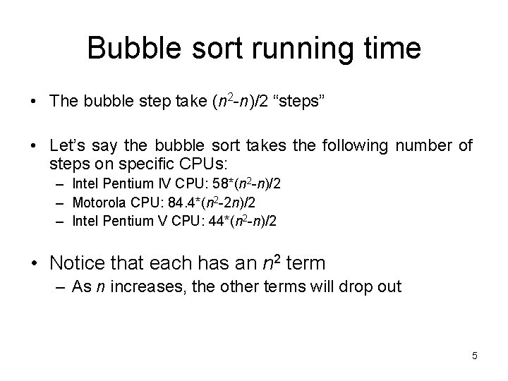
Bubble sort running time • The bubble step take (n 2 -n)/2 “steps” • Let’s say the bubble sort takes the following number of steps on specific CPUs: – Intel Pentium IV CPU: 58*(n 2 -n)/2 – Motorola CPU: 84. 4*(n 2 -2 n)/2 – Intel Pentium V CPU: 44*(n 2 -n)/2 • Notice that each has an n 2 term – As n increases, the other terms will drop out 5

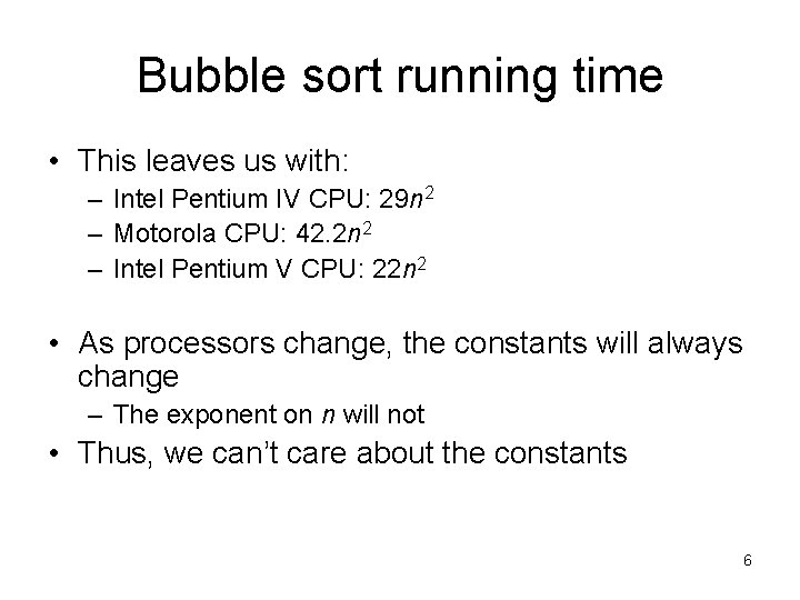
Bubble sort running time • This leaves us with: – Intel Pentium IV CPU: 29 n 2 – Motorola CPU: 42. 2 n 2 – Intel Pentium V CPU: 22 n 2 • As processors change, the constants will always change – The exponent on n will not • Thus, we can’t care about the constants 6

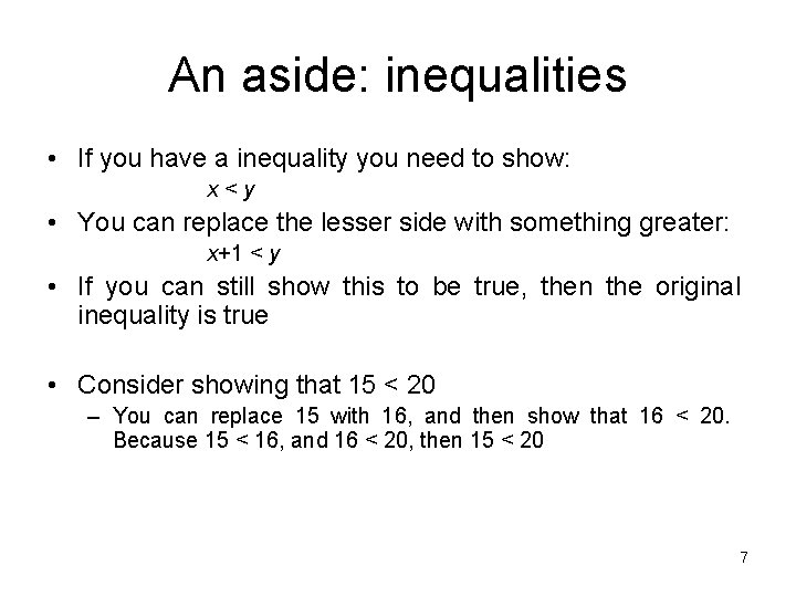
An aside: inequalities • If you have a inequality you need to show: x<y • You can replace the lesser side with something greater: x+1 < y • If you can still show this to be true, then the original inequality is true • Consider showing that 15 < 20 – You can replace 15 with 16, and then show that 16 < 20. Because 15 < 16, and 16 < 20, then 15 < 20 7

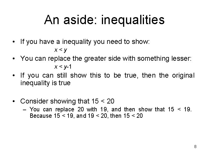
An aside: inequalities • If you have a inequality you need to show: x<y • You can replace the greater side with something lesser: x < y-1 • If you can still show this to be true, then the original inequality is true • Consider showing that 15 < 20 – You can replace 20 with 19, and then show that 15 < 19. Because 15 < 19, and 19 < 20, then 15 < 20 8

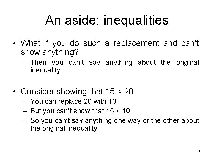
An aside: inequalities • What if you do such a replacement and can’t show anything? – Then you can’t say anything about the original inequality • Consider showing that 15 < 20 – You can replace 20 with 10 – But you can’t show that 15 < 10 – So you can’t say anything one way or the other about the original inequality 9

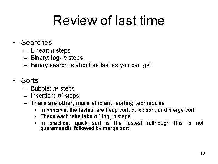
Review of last time • Searches – Linear: n steps – Binary: log 2 n steps – Binary search is about as fast as you can get • Sorts – Bubble: n 2 steps – Insertion: n 2 steps – There are other, more efficient, sorting techniques • In principle, the fastest are heap sort, quick sort, and merge sort • These each take n * log 2 n steps • In practice, quick sort is the fastest (although this is not guaranteed!), followed by merge sort 10

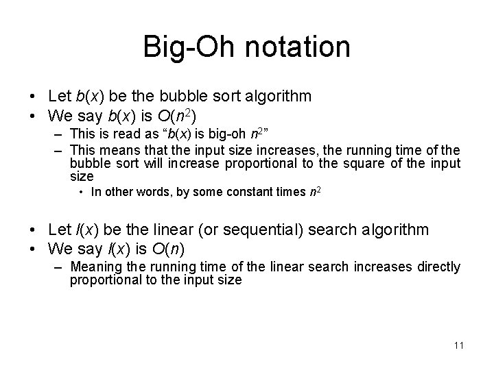
Big-Oh notation • Let b(x) be the bubble sort algorithm • We say b(x) is O(n 2) – This is read as “b(x) is big-oh n 2” – This means that the input size increases, the running time of the bubble sort will increase proportional to the square of the input size • In other words, by some constant times n 2 • Let l(x) be the linear (or sequential) search algorithm • We say l(x) is O(n) – Meaning the running time of the linear search increases directly proportional to the input size 11

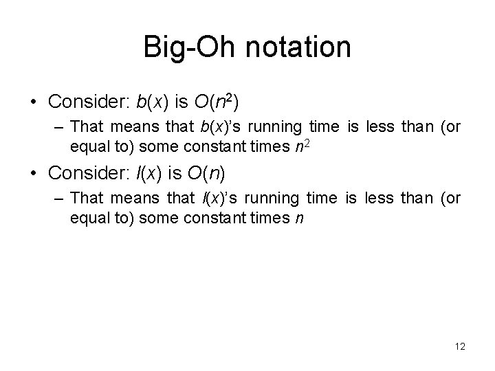
Big-Oh notation • Consider: b(x) is O(n 2) – That means that b(x)’s running time is less than (or equal to) some constant times n 2 • Consider: l(x) is O(n) – That means that l(x)’s running time is less than (or equal to) some constant times n 12

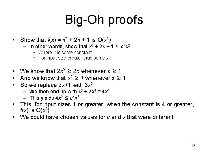
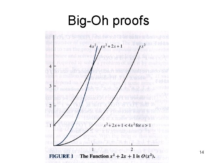
Big-Oh proofs • Show that f(x) = x 2 + 2 x + 1 is O(x 2) – In other words, show that x 2 + 2 x + 1 ≤ c*x 2 • Where c is some constant • For input size greater than some x • We know that 2 x 2 ≥ 2 x whenever x ≥ 1 • And we know that x 2 ≥ 1 whenever x ≥ 1 • So we replace 2 x+1 with 3 x 2 – We then end up with x 2 + 3 x 2 = 4 x 2 – This yields 4 x 2 ≤ c*x 2 • This, for input sizes 1 or greater, when the constant is 4 or greater, f(x) is O(x 2) • We could have chosen values for c and x that were different 13

Big-Oh proofs 14

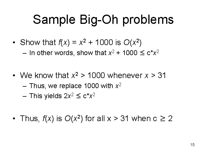
Sample Big-Oh problems • Show that f(x) = x 2 + 1000 is O(x 2) – In other words, show that x 2 + 1000 ≤ c*x 2 • We know that x 2 > 1000 whenever x > 31 – Thus, we replace 1000 with x 2 – This yields 2 x 2 ≤ c*x 2 • Thus, f(x) is O(x 2) for all x > 31 when c ≥ 2 15

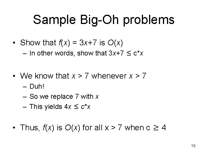
Sample Big-Oh problems • Show that f(x) = 3 x+7 is O(x) – In other words, show that 3 x+7 ≤ c*x • We know that x > 7 whenever x > 7 – Duh! – So we replace 7 with x – This yields 4 x ≤ c*x • Thus, f(x) is O(x) for all x > 7 when c ≥ 4 16

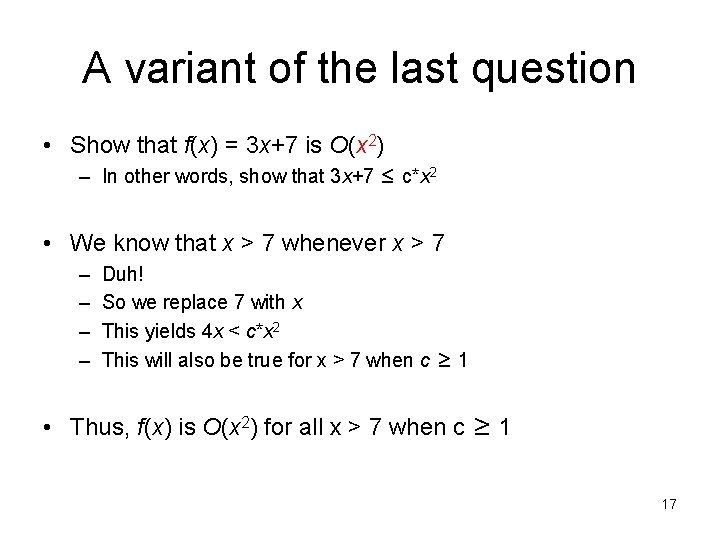
A variant of the last question • Show that f(x) = 3 x+7 is O(x 2) – In other words, show that 3 x+7 ≤ c*x 2 • We know that x > 7 whenever x > 7 – – Duh! So we replace 7 with x This yields 4 x < c*x 2 This will also be true for x > 7 when c ≥ 1 • Thus, f(x) is O(x 2) for all x > 7 when c ≥ 1 17

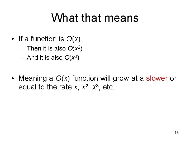
What that means • If a function is O(x) – Then it is also O(x 2) – And it is also O(x 3) • Meaning a O(x) function will grow at a slower or equal to the rate x, x 2, x 3, etc. 18

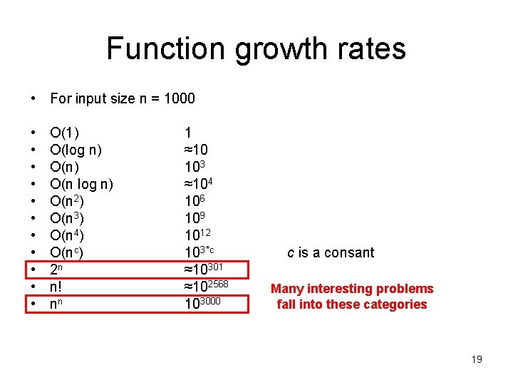
Function growth rates • For input size n = 1000 • • • O(1) O(log n) O(n 2) O(n 3) O(n 4) O(nc) 2 n n! nn 1 ≈10 103 ≈104 106 109 1012 103*c ≈10301 ≈102568 103000 c is a consant Many interesting problems fall into these categories 19

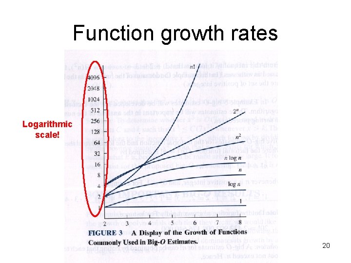
Function growth rates Logarithmic scale! 20

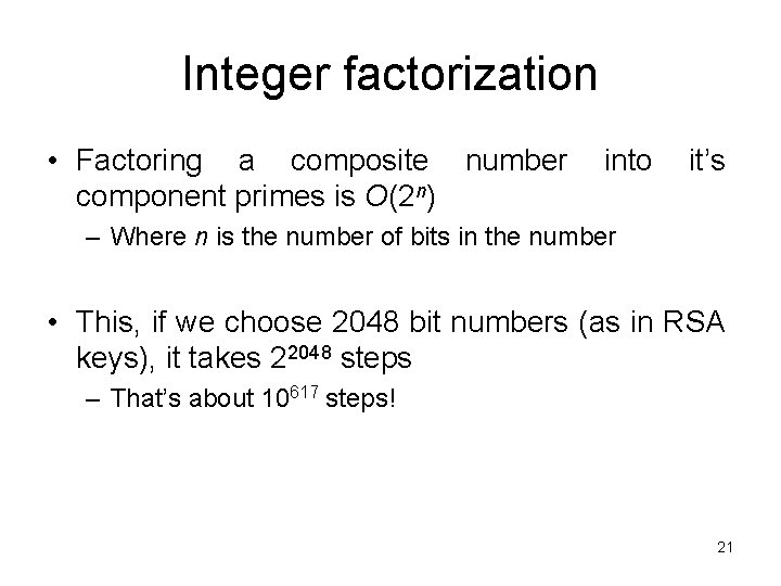
Integer factorization • Factoring a composite number component primes is O(2 n) into it’s – Where n is the number of bits in the number • This, if we choose 2048 bit numbers (as in RSA keys), it takes 22048 steps – That’s about 10617 steps! 21

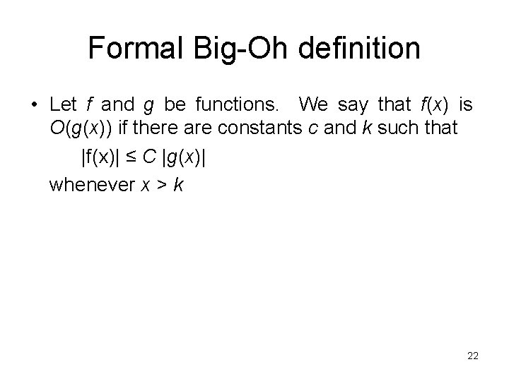
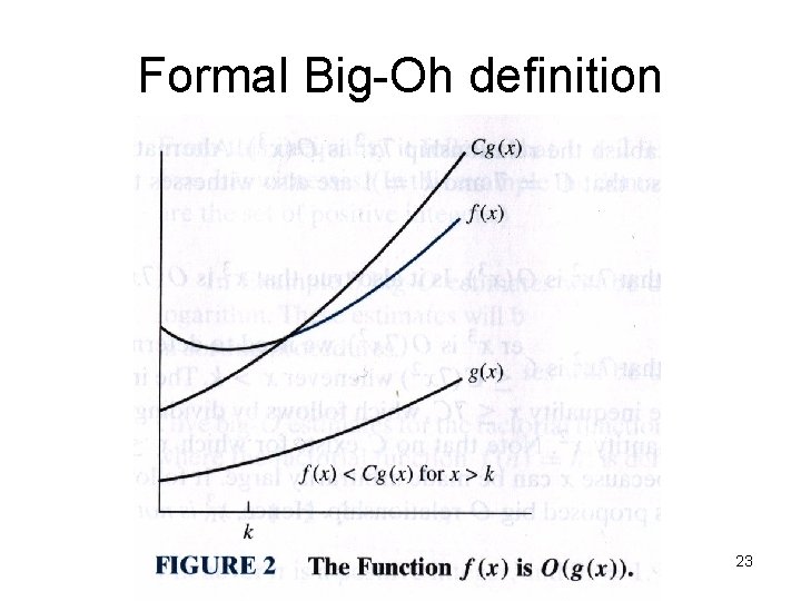
Formal Big-Oh definition • Let f and g be functions. We say that f(x) is O(g(x)) if there are constants c and k such that |f(x)| ≤ C |g(x)| whenever x > k 22

Formal Big-Oh definition 23

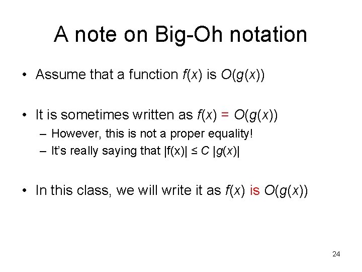
A note on Big-Oh notation • Assume that a function f(x) is O(g(x)) • It is sometimes written as f(x) = O(g(x)) – However, this is not a proper equality! – It’s really saying that |f(x)| ≤ C |g(x)| • In this class, we will write it as f(x) is O(g(x)) 24

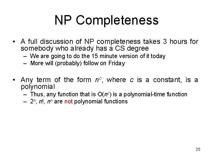
NP Completeness • A full discussion of NP completeness takes 3 hours for somebody who already has a CS degree – We are going to do the 15 minute version of it today – More will (probably) follow on Friday • Any term of the form nc, where c is a constant, is a polynomial – Thus, any function that is O(nc) is a polynomial-time function – 2 n, n!, nn are not polynomial functions 25

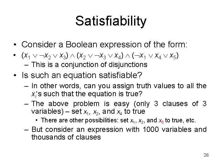
Satisfiability • Consider a Boolean expression of the form: • (x 1 x 2 x 3) (x 2 x 3 x 4) ( x 1 x 4 x 5) – This is a conjunction of disjunctions • Is such an equation satisfiable? – In other words, can you assign truth values to all the xi’s such that the equation is true? – The above problem is easy (only 3 clauses of 3 variables) – set x 1, x 2, and x 4 to true • There are other possibilities: set x 1, x 2, and x 5 to true, etc. – But consider an expression with 1000 variables and thousands of clauses 26

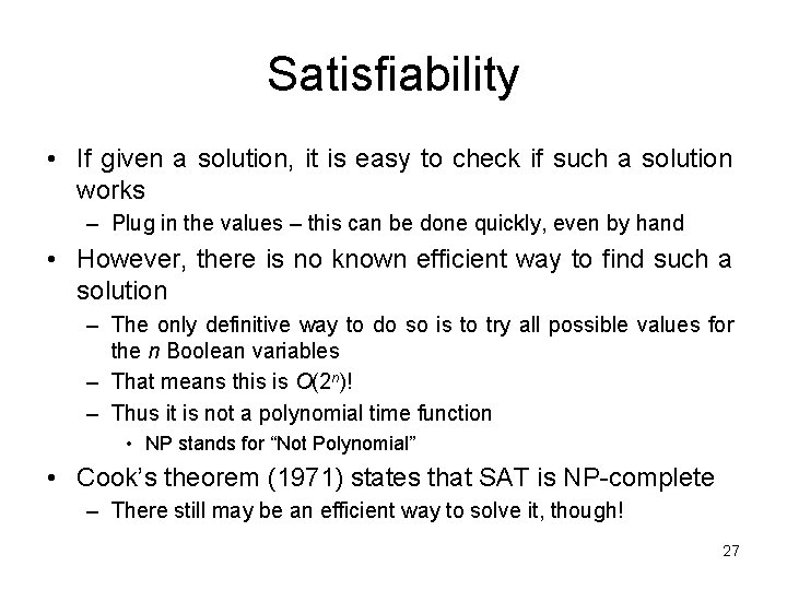
Satisfiability • If given a solution, it is easy to check if such a solution works – Plug in the values – this can be done quickly, even by hand • However, there is no known efficient way to find such a solution – The only definitive way to do so is to try all possible values for the n Boolean variables – That means this is O(2 n)! – Thus it is not a polynomial time function • NP stands for “Not Polynomial” • Cook’s theorem (1971) states that SAT is NP-complete – There still may be an efficient way to solve it, though! 27

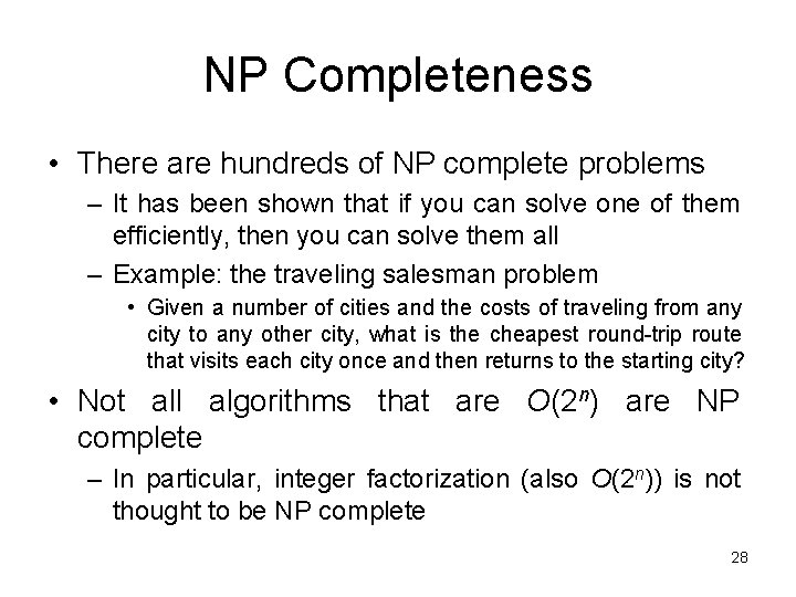
NP Completeness • There are hundreds of NP complete problems – It has been shown that if you can solve one of them efficiently, then you can solve them all – Example: the traveling salesman problem • Given a number of cities and the costs of traveling from any city to any other city, what is the cheapest round-trip route that visits each city once and then returns to the starting city? • Not all algorithms that are O(2 n) are NP complete – In particular, integer factorization (also O(2 n)) is not thought to be NP complete 28

NP Completeness • It is “widely believed” that there is no efficient solution to NP complete problems – In other words, everybody has that belief • If you could solve an NP complete problem in polynomial time, you would be showing that P = NP – And you’d get a million dollar prize (and lots of fame!) • If this were possible, it would be like proving that Newton’s or Einstein’s laws of physics were wrong • In summary: – NP complete problems are very difficult to solve, but easy to check the solutions of – It is believed that there is no efficient way to solve them 29