Growth Curve Model Using SEM David A Kenny

Growth Curve Model Using SEM David A. Kenny December 15, 2013

Thanks due to Betsy Mc. Coach

Linear Growth Curve Models • We have at least three time points for each individual. • We fit a straight line for each person: • The parameters from these lines describe the person. • Nonlinear growth models are possible. 3

The Key Parameters • Slope: the rate of change – Some people are changing more than others and so have larger slopes. – Some people are improving or growing (positive slopes). – Some are declining (negative slopes). – Some are not changing (zero slopes). • Intercept: where the person starts • Error: How far the score is from the line. 4

Latent Growth Models (LGM) • For both the slope and intercept there is a mean and a variance. – Mean • Intercept: Where does the average person start? • Slope: What is the average rate of change? – Variance • Intercept: How much do individuals differ in where they start? • Slope: How much do individuals differ in their rates of change: “Different slopes for different folks. ” 5

Measurement Over Time • measures taken over time – chronological time: 2006, 2007, 2008 – personal time: 5 years old, 6, and 7 • missing data not problematic – person fails to show up at age 6 • unequal spacing of observations not problematic – measures at 2000, 2001, 2002, and 2006 6

Data • Types – Raw data – Covariance matrix plus means Means become knowns: T(T + 3)/2 Should not use CFI and TLI (unless the independence model is recomputed; zero correlations, free variances, means equal) • Program reproduces variances, covariances (correlations), and means. 7

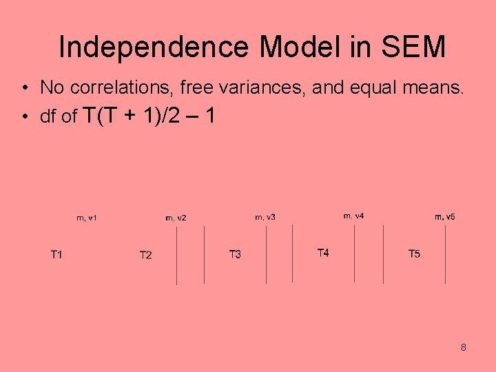
Independence Model in SEM • No correlations, free variances, and equal means. • df of T(T + 1)/2 – 1 8

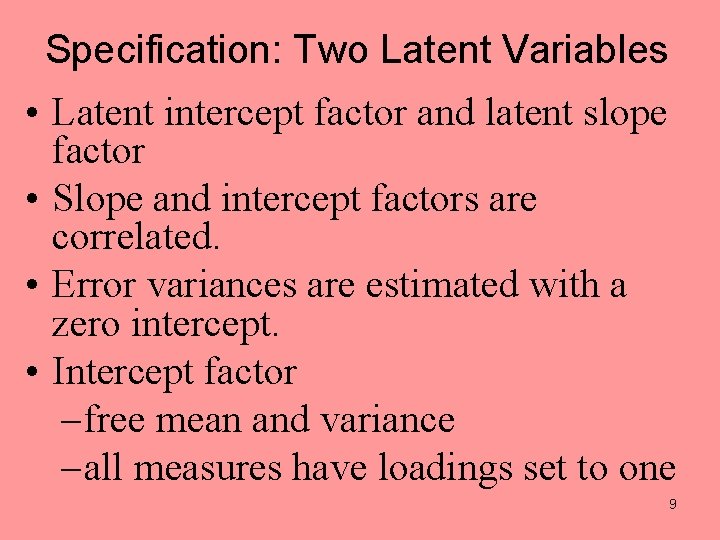
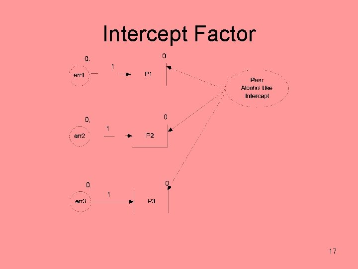
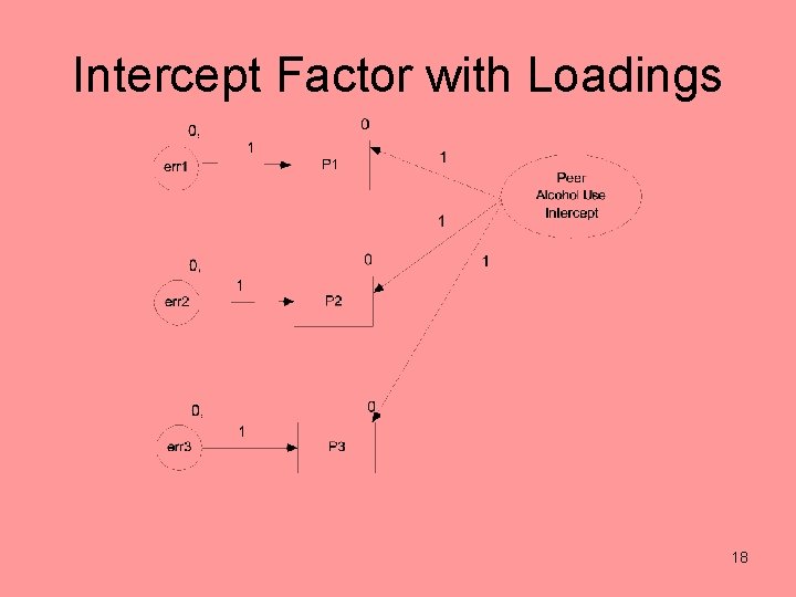
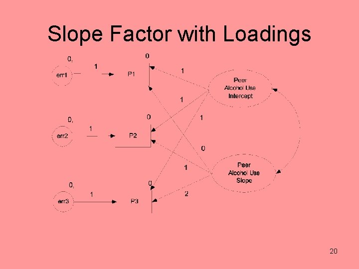
Specification: Two Latent Variables • Latent intercept factor and latent slope factor • Slope and intercept factors are correlated. • Error variances are estimated with a zero intercept. • Intercept factor – free mean and variance – all measures have loadings set to one 9

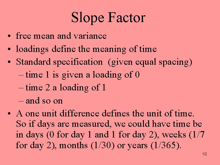
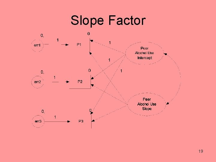
Slope Factor • free mean and variance • loadings define the meaning of time • Standard specification (given equal spacing) – time 1 is given a loading of 0 – time 2 a loading of 1 – and so on • A one unit difference defines the unit of time. So if days are measured, we could have time be in days (0 for day 1 and 1 for day 2), weeks (1/7 for day 2), months (1/30) or years (1/365). 10

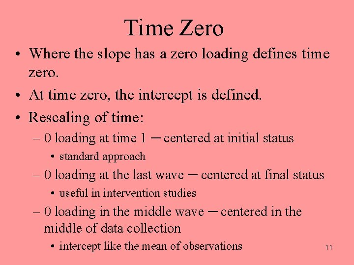
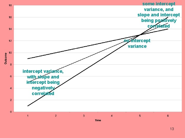
Time Zero • Where the slope has a zero loading defines time zero. • At time zero, the intercept is defined. • Rescaling of time: – 0 loading at time 1 ─ centered at initial status • standard approach – 0 loading at the last wave ─ centered at final status • useful in intervention studies – 0 loading in the middle wave ─ centered in the middle of data collection • intercept like the mean of observations 11

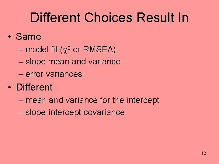
Different Choices Result In • Same – model fit (c 2 or RMSEA) – slope mean and variance – error variances • Different – mean and variance for the intercept – slope-intercept covariance 12

some intercept variance, and slope and intercept being positively correlated no intercept variance, with slope and intercept being negatively correlated 13

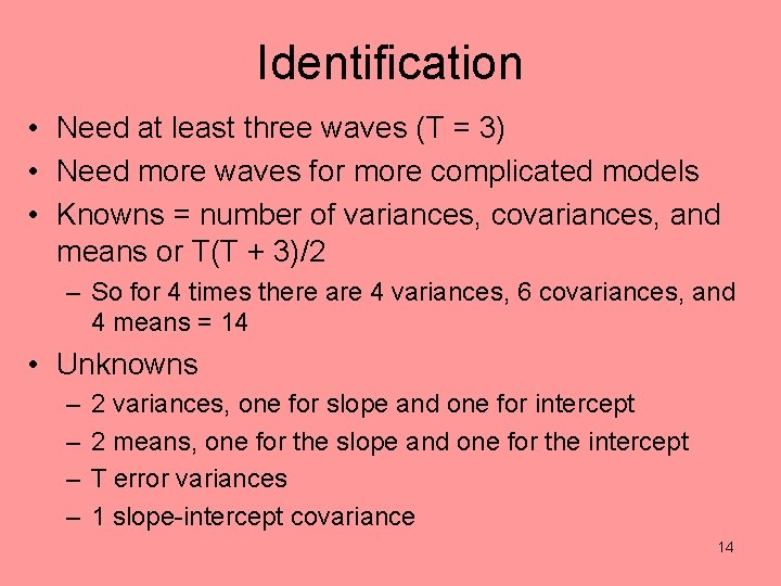
Identification • Need at least three waves (T = 3) • Need more waves for more complicated models • Knowns = number of variances, covariances, and means or T(T + 3)/2 – So for 4 times there are 4 variances, 6 covariances, and 4 means = 14 • Unknowns – – 2 variances, one for slope and one for intercept 2 means, one for the slope and one for the intercept T error variances 1 slope-intercept covariance 14

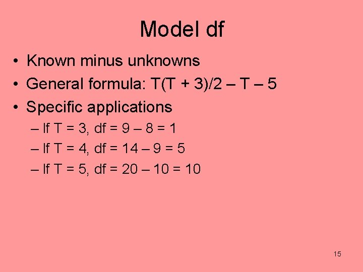
Model df • Known minus unknowns • General formula: T(T + 3)/2 – T – 5 • Specific applications – If T = 3, df = 9 – 8 = 1 – If T = 4, df = 14 – 9 = 5 – If T = 5, df = 20 – 10 = 10 15

Three-wave Model • Has one df. • The over-identifying restriction is: M 1 + M 3 – 2 M 2 = 0 (where “M” is mean) i. e. , the means have a linear relationship with respect to time. 16

Intercept Factor 17

Intercept Factor with Loadings 18

Slope Factor 19

Slope Factor with Loadings 20

Alternative Options for Error Variances • Force error variances to be equal across time. • Non-independent errors – errors of adjacent waves correlated – autoregressive errors (err 1 err 2 err 3) 21

Trimming Growth Curve Models • Almost never trim – Slope-intercept covariance – Intercept variance • Never have the intercept “cause” the slope factor or vice versa. • Slope variance: OK to trim, i. e. , set to zero. – If trimmed set slope-intercept covariance to zero. • Do not interpret standardized estimates except the slope-intercept correlation. 22

Relationship to Multilevel Modeling (MLM) • Equivalent if ML option is chosen • Advantages of SEM – Measures of absolute fit – Easier to respecify; more options for respecification – More flexibility in the error covariance structure – Easier to specify changes in slope loadings over time – Allows latent covariates – Allows missing data in covariates • Advantages of MLM – Better with time-unstructured data – Easier with many times – Better with fewer participants – Easier with time-varying covariates – Random effects of time-varying covariates allowable 23