Grouping What is grouping Kmeans Input set of

Grouping

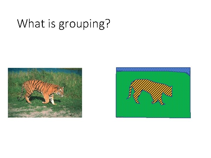
What is grouping?

K-means Input: set of data points, k 1. Randomly pick k points as means 2. For i in [0, maxiters]: 1. Assign each point to nearest center 2. Re-estimate each center as mean of points assigned to it

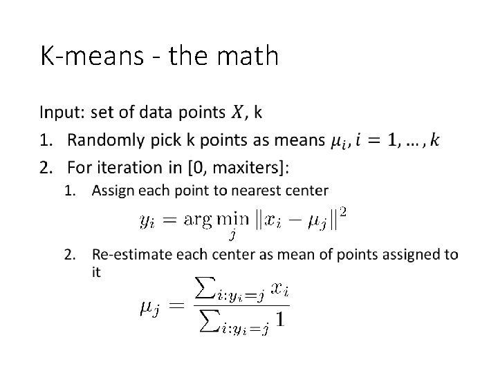
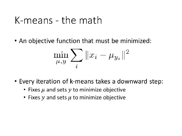
K-means - the math •

K-means - the math •

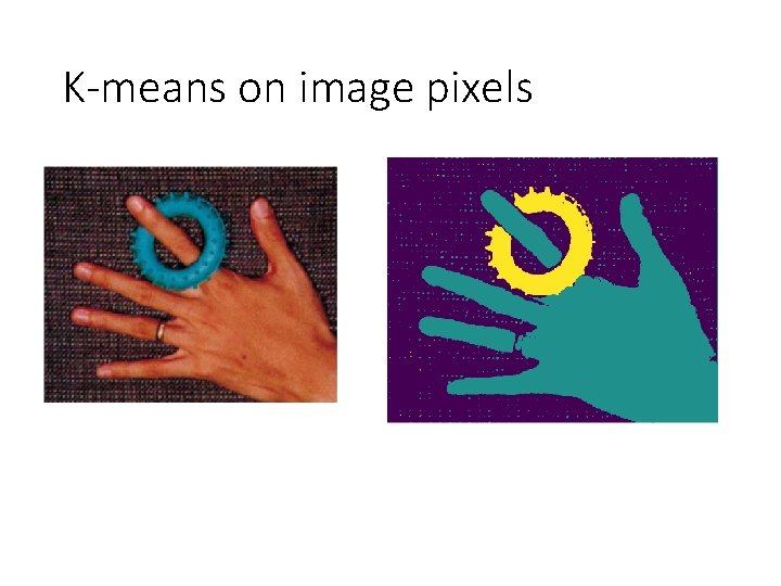
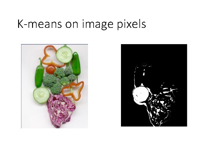
K-means on image pixels

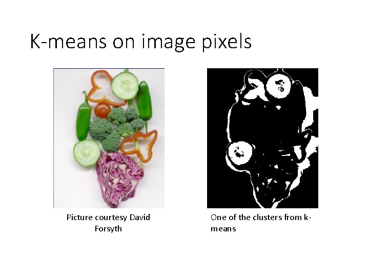
K-means on image pixels Picture courtesy David Forsyth One of the clusters from kmeans

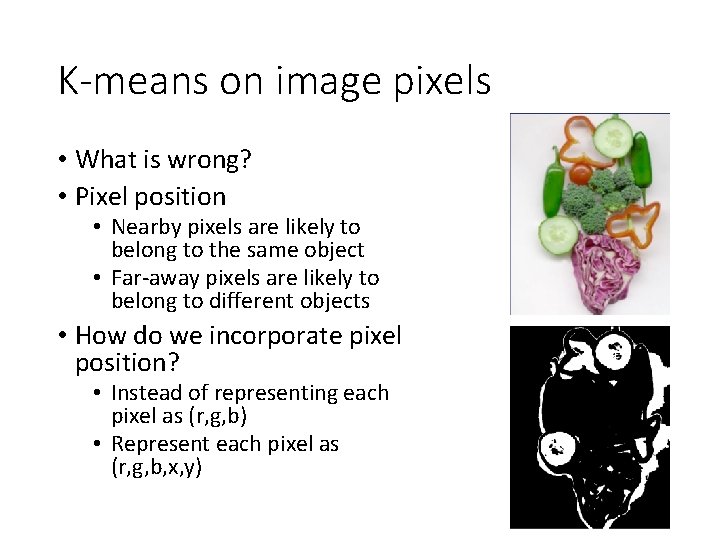
K-means on image pixels • What is wrong? • Pixel position • Nearby pixels are likely to belong to the same object • Far-away pixels are likely to belong to different objects • How do we incorporate pixel position? • Instead of representing each pixel as (r, g, b) • Represent each pixel as (r, g, b, x, y)

K-means on image pixels

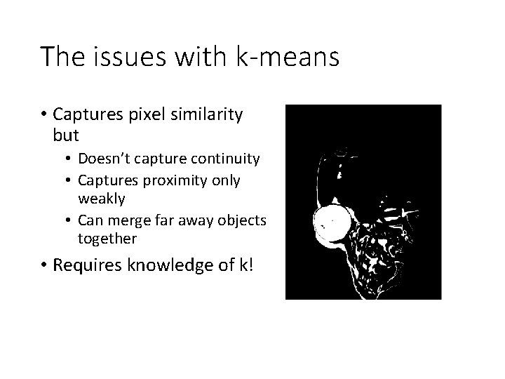
The issues with k-means • Captures pixel similarity but • Doesn’t capture continuity • Captures proximity only weakly • Can merge far away objects together • Requires knowledge of k!

Oversegmentation and superpixels • We don’t know k. What is a safe choice? • Idea: Use large k • Can potentially break big objects, but will hopefully not merge unrelated objects • Later processing can decide which groups to merge • Called superpixels

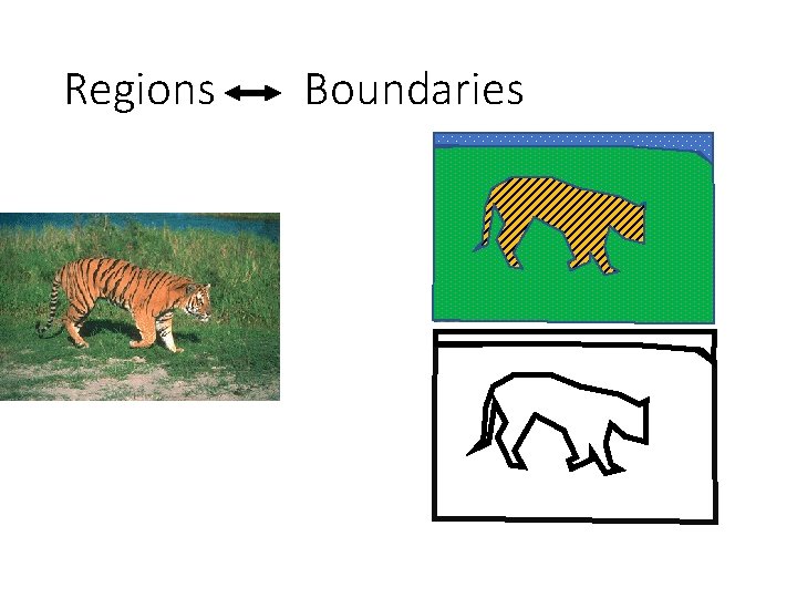
Regions Boundaries

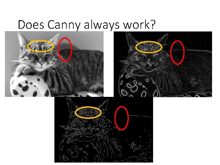
Does Canny always work?

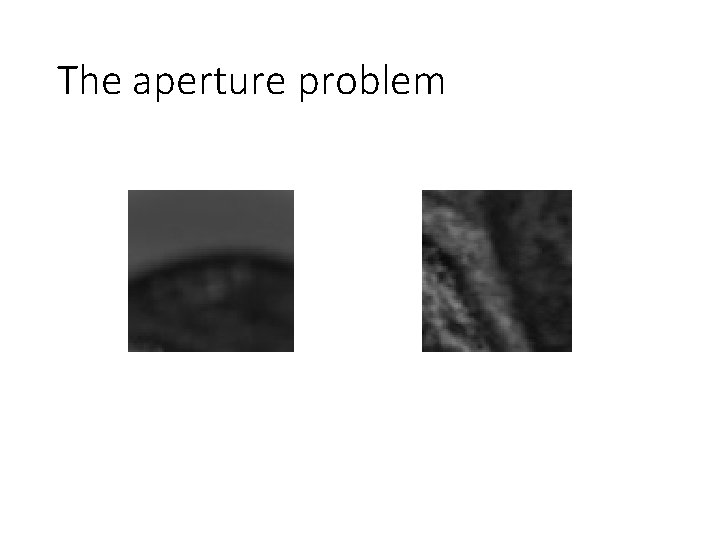
The aperture problem

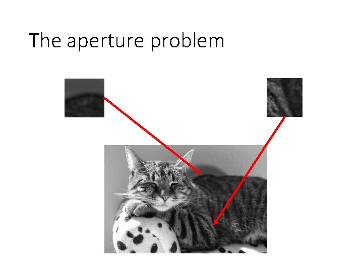
The aperture problem

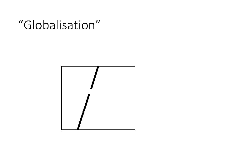
“Globalisation”

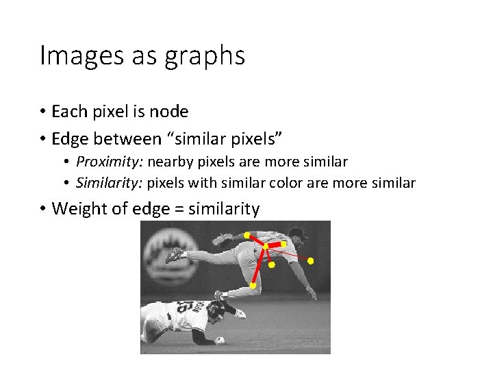
Images as graphs • Each pixel is node • Edge between “similar pixels” • Proximity: nearby pixels are more similar • Similarity: pixels with similar color are more similar • Weight of edge = similarity

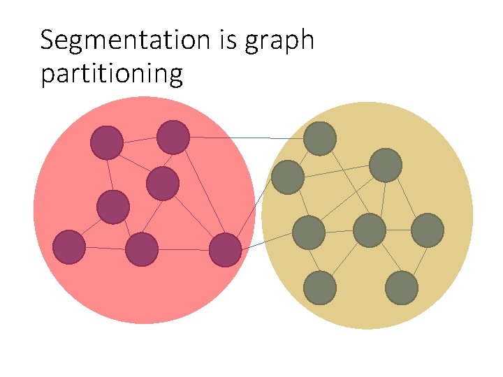
Segmentation is graph partitioning

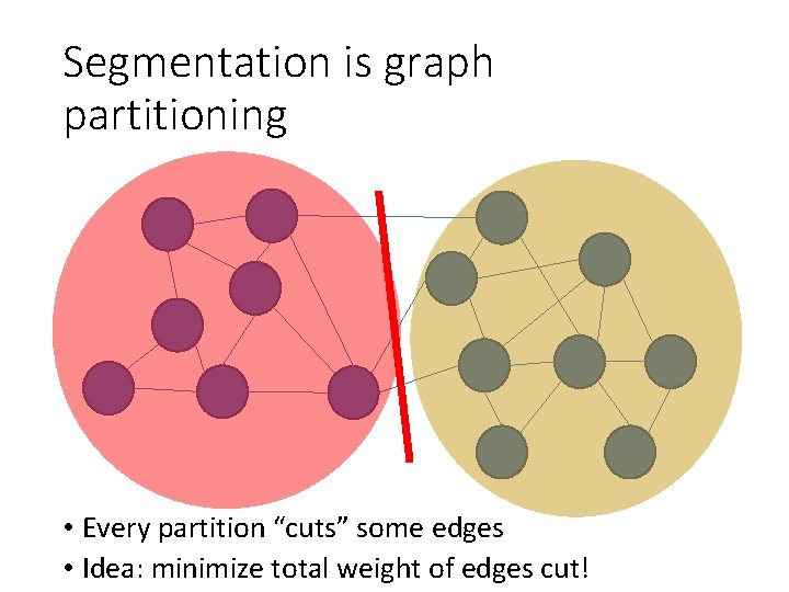
Segmentation is graph partitioning • Every partition “cuts” some edges • Idea: minimize total weight of edges cut!

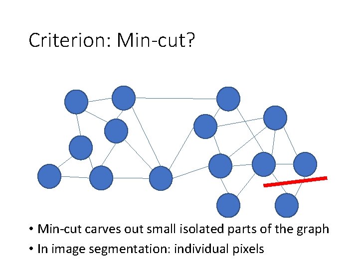
Criterion: Min-cut? • Min-cut carves out small isolated parts of the graph • In image segmentation: individual pixels

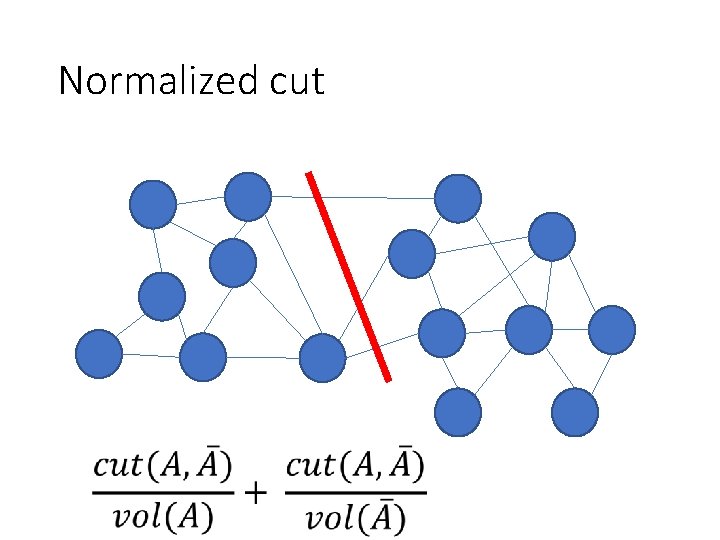
Normalized cuts • “Cut” = total weight of cut edges • Small cut means the groups don’t “like” each other • But need to normalize w. r. t how much they like themselves • “Volume” of a subgraph = total weight of edges within the subgraph

Normalized cut

Min-cut vs normalized cut • Both rely on interpreting images as graphs • By itself, min-cut gives small isolated pixels • But can work if we add other constraints • min-cut can be solved in polynomial time • Dual of max-flow • N-cut is NP-hard • But approximations exist!

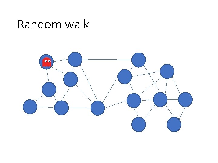
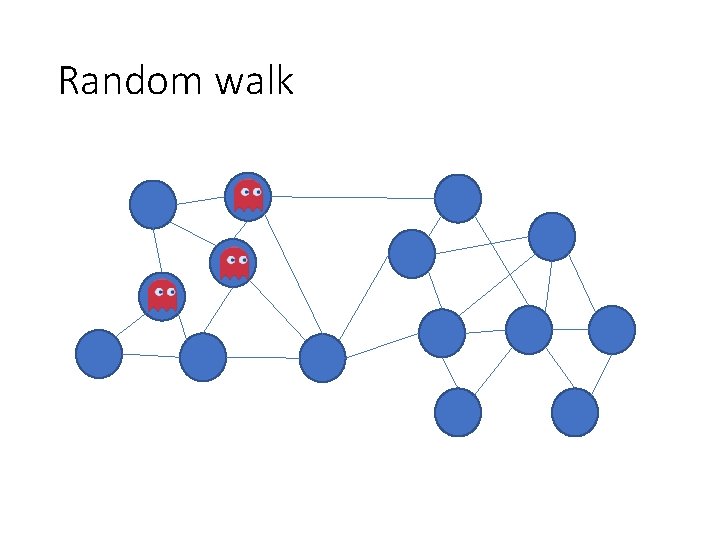
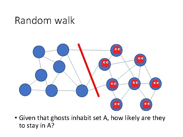
Random walk

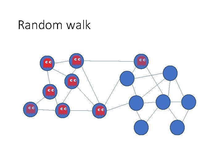
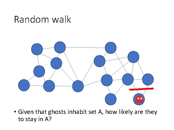
Random walk

Random walk

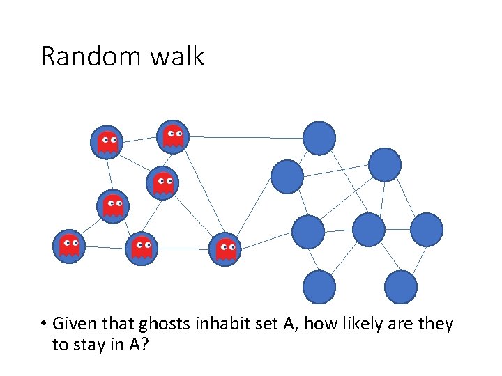
Random walk • Given that ghosts inhabit set A, how likely are they to stay in A?

Random walk • Given that ghosts inhabit set A, how likely are they to stay in A?

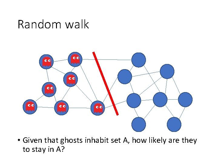
Random walk • Given that ghosts inhabit set A, how likely are they to stay in A?

Random walk • Given that ghosts inhabit set A, how likely are they to stay in A?

Random walk • Key idea: Partition should be such that ghost should be likely to stay in one partition • Normalized cut criterion is the same as this • But how do we find this partition?

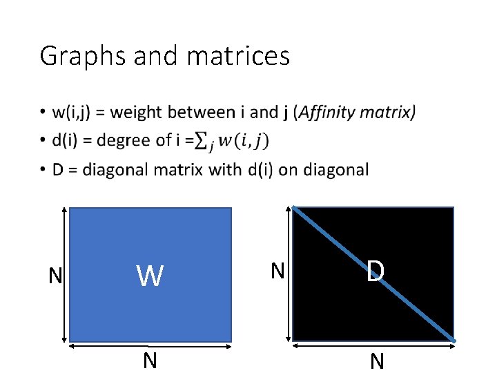
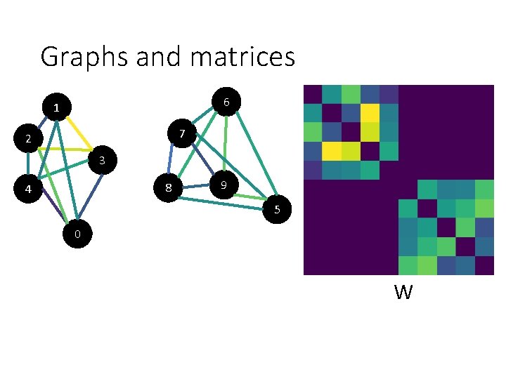
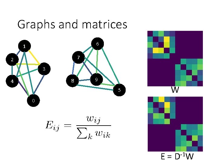
Graphs and matrices • N W N N D N

Graphs and matrices 6 1 7 2 3 8 4 9 5 0 W

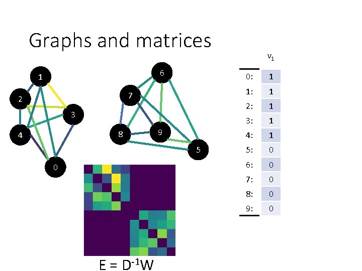
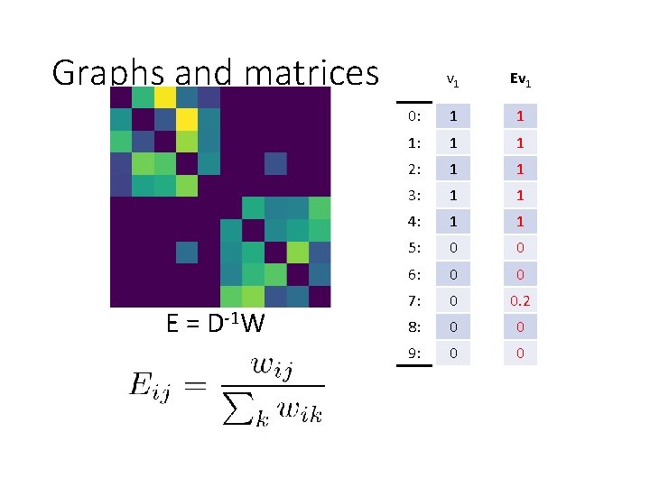
Graphs and matrices 6 1 7 2 3 8 4 9 5 W 0 E = D-1 W

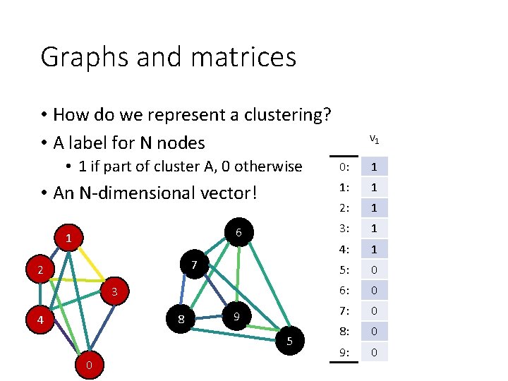
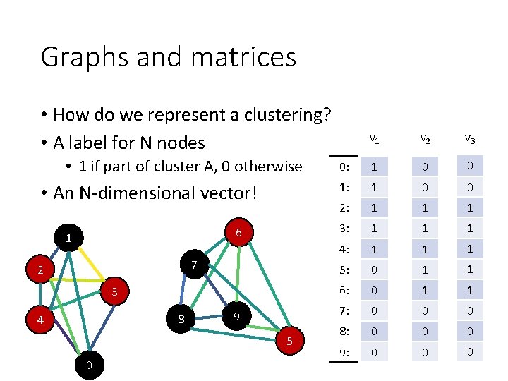
Graphs and matrices • How do we represent a clustering? • A label for N nodes • 1 if part of cluster A, 0 otherwise • An N-dimensional vector! 6 1 7 2 3 8 4 9 5 0 v 1 0: 1 1: 1 2: 1 3: 1 4: 1 5: 0 6: 0 7: 0 8: 0 9: 0

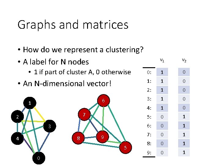
Graphs and matrices • How do we represent a clustering? • A label for N nodes • 1 if part of cluster A, 0 otherwise • An N-dimensional vector! 6 1 7 2 3 8 4 9 5 0 v 1 v 2 0: 1 0 1: 1 0 2: 1 0 3: 1 0 4: 1 0 5: 0 1 6: 0 1 7: 0 1 8: 0 1 9: 0 1

Graphs and matrices • How do we represent a clustering? • A label for N nodes • 1 if part of cluster A, 0 otherwise • An N-dimensional vector! 6 1 7 2 3 8 4 9 5 0 v 1 v 2 v 3 0: 1 0 0 1: 1 0 0 2: 1 1 1 3: 1 1 1 4: 1 1 1 5: 0 1 1 6: 0 1 1 7: 0 0 0 8: 0 0 0 9: 0 0 0

Graphs and matrices 6 1 7 2 3 8 4 9 5 0 E = D-1 W v 1 0: 1 1: 1 2: 1 3: 1 4: 1 5: 0 6: 0 7: 0 8: 0 9: 0

Graphs and matrices E = D-1 W v 1 Ev 1 0: 1 1 1: 1 1 2: 1 1 3: 1 1 4: 1 1 5: 0 0 6: 0 0 7: 0 0 8: 0 0 9: 0 0

Graphs and matrices E = D-1 W v 2 Ev 2 0: 0 0 1: 0 0 2: 0 0 3: 0 0 4: 0 0 5: 1 1 6: 1 1 7: 1 1 8: 1 1 9: 1 1

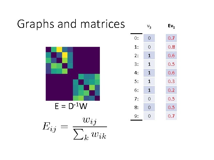
Graphs and matrices E = D-1 W v 3 Ev 3 0: 0 0. 7 1: 0 0. 8 2: 1 0. 6 3: 1 0. 5 4: 1 0. 6 5: 1 0. 3 6: 1 0. 2 7: 0 0. 5 8: 0 0. 5 9: 0 0. 7

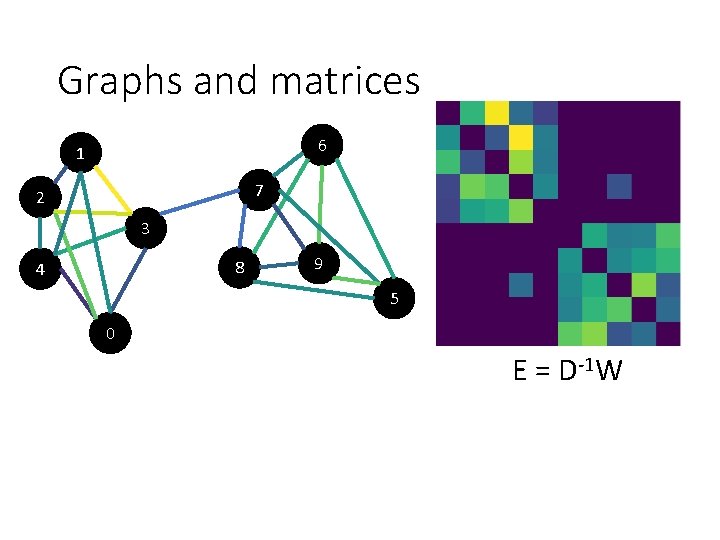
Graphs and matrices 6 1 7 2 3 8 4 9 5 0 E = D-1 W

Graphs and matrices E = D-1 W v 1 Ev 1 0: 1 1 1: 1 1 2: 1 1 3: 1 1 4: 1 1 5: 0 0 6: 0 0 7: 0 0. 2 8: 0 0 9: 0 0

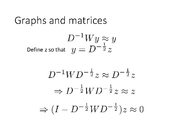
Graphs and matrices Define z so that

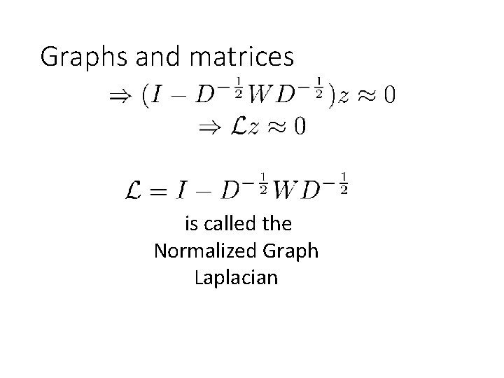
Graphs and matrices is called the Normalized Graph Laplacian

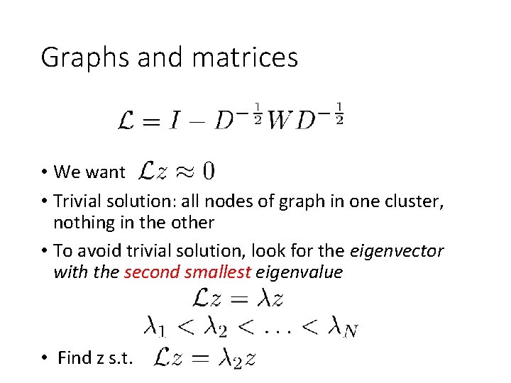
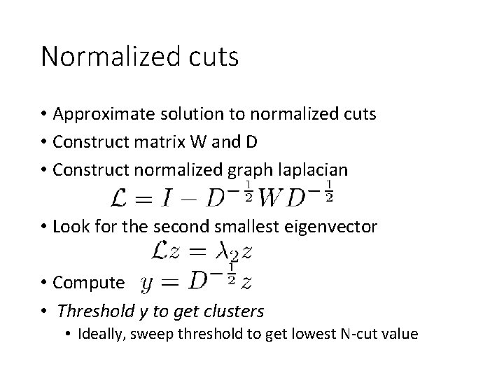
Graphs and matrices • We want • Trivial solution: all nodes of graph in one cluster, nothing in the other • To avoid trivial solution, look for the eigenvector with the second smallest eigenvalue • Find z s. t.

Normalized cuts • Approximate solution to normalized cuts • Construct matrix W and D • Construct normalized graph laplacian • Look for the second smallest eigenvector • Compute • Threshold y to get clusters • Ideally, sweep threshold to get lowest N-cut value

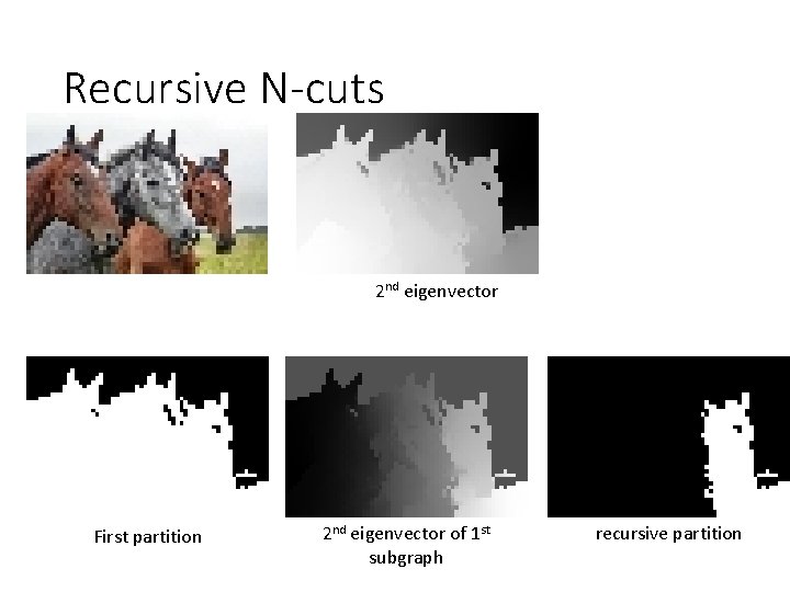
More than 2 clusters • Given graph, use N-cuts to get 2 clusters • Each cluster is a graph • Re-run N-cuts on each graph

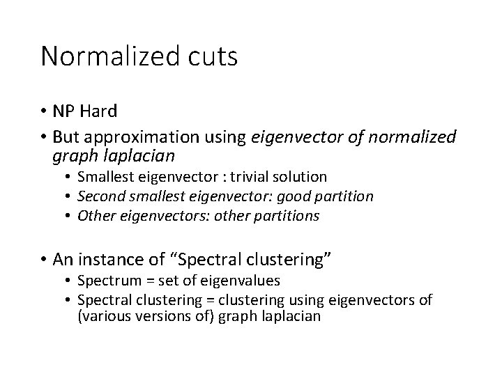
Normalized cuts • NP Hard • But approximation using eigenvector of normalized graph laplacian • Smallest eigenvector : trivial solution • Second smallest eigenvector: good partition • Other eigenvectors: other partitions • An instance of “Spectral clustering” • Spectrum = set of eigenvalues • Spectral clustering = clustering using eigenvectors of (various versions of) graph laplacian

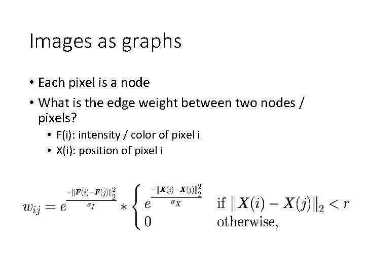
Images as graphs • Each pixel is a node • What is the edge weight between two nodes / pixels? • F(i): intensity / color of pixel i • X(i): position of pixel i

Computational complexity • A 100 x 100 image has 10 K pixels • A graph with 10 K pixels has a 10 K x 10 K affinity matrix • Eigenvalue computation of an N x N matrix is O(N 3) • Very very expensive!

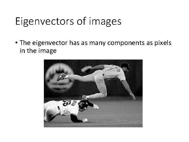
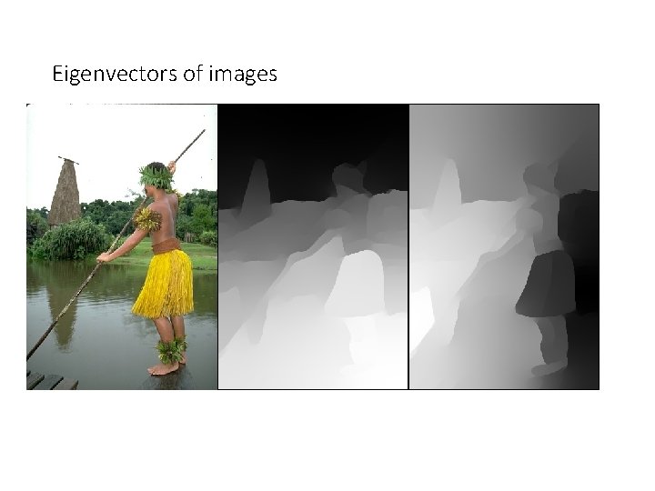
Eigenvectors of images • The eigenvector has as many components as pixels in the image

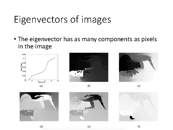
Eigenvectors of images • The eigenvector has as many components as pixels in the image

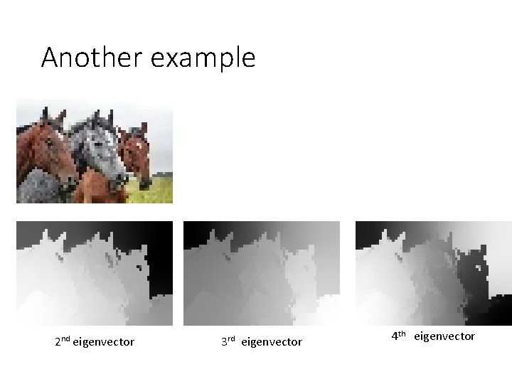
Another example 2 nd eigenvector 3 rd eigenvector 4 th eigenvector

Recursive N-cuts 2 nd eigenvector First partition 2 nd eigenvector of 1 st subgraph recursive partition

N-Cuts resources • http: //scikitlearn. org/stable/modules/clustering. html#spectralclustering • https: //people. eecs. berkeley. edu/~malik/papers/S M-ncut. pdf

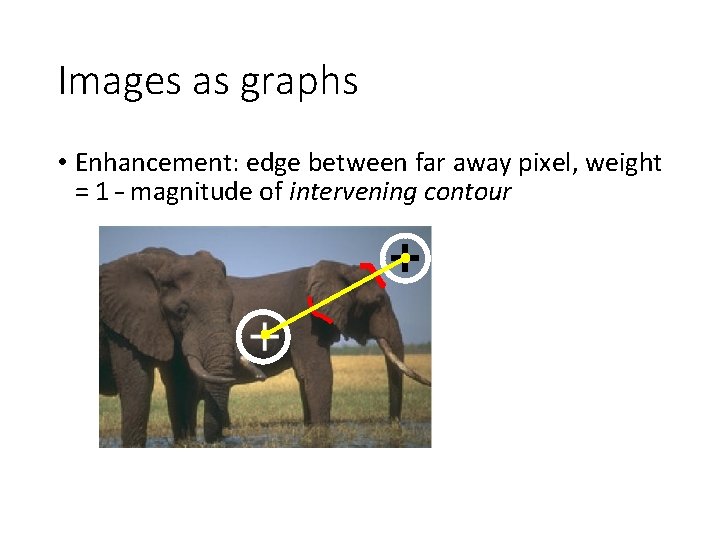
Images as graphs • Enhancement: edge between far away pixel, weight = 1 – magnitude of intervening contour

Eigenvectors of images