Group Examples Domain selections spatial and temporal Calculate

- Slides: 26

Group Examples • Domain selections (spatial and temporal) • Calculate… – – Climatologies Anomalies Spatial averages Seasonal averages • Customize maps/graphs • Create data masks • Prep data files for analysis in CPT

Group Example 1 • Use Datasets by Category catalog to find a data set with the following characteristics: 1. Includes observed sea surface temperatures 2. Monthly temporal resolution 3. Spatial resolution at least 1ºx 1º 4. Includes 60ºS-60ºN in spatial domain 5. Includes 1985 -2005 in temporal domain

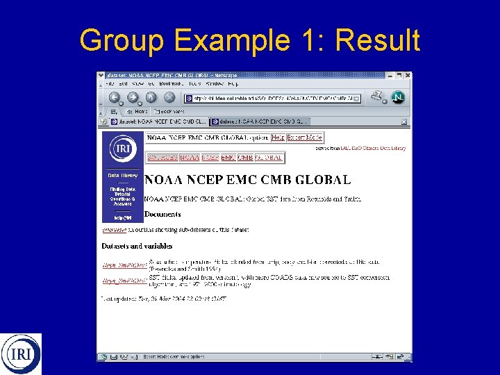
Group Example 1: Result

Group Example 2: Prepare spatially averaged monthly SSTs in the Tropical Atlantic region for 1986 -2005 for use in Excel • From the Reyn_Smith. OIv 2 monthly data… – – – – START HERE Select the Sea Surface Temperature variable Select Jan 1986 – Dec 2005 time period Select region in Tropical Atlantic (10ºS-10ºN, 330ºE-350ºE) Calculate spatial average (XY link on Filters page) View Ingrid in Expert Mode View data in data viewer Download for use in Excel

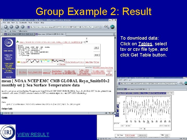
Group Example 2: Result To download data: Click on Tables, select tsv or csv file type, and click Get Table button. VIEW RESULT

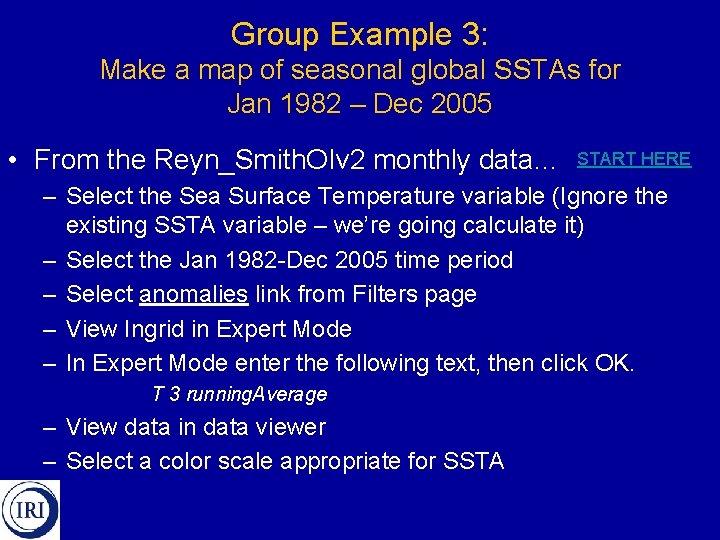
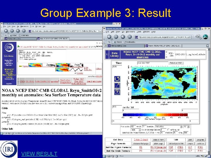
Group Example 3: Make a map of seasonal global SSTAs for Jan 1982 – Dec 2005 • From the Reyn_Smith. OIv 2 monthly data… START HERE – Select the Sea Surface Temperature variable (Ignore the existing SSTA variable – we’re going calculate it) – Select the Jan 1982 -Dec 2005 time period – Select anomalies link from Filters page – View Ingrid in Expert Mode – In Expert Mode enter the following text, then click OK. T 3 running. Average – View data in data viewer – Select a color scale appropriate for SSTA

Group Example 3: Result VIEW RESULT

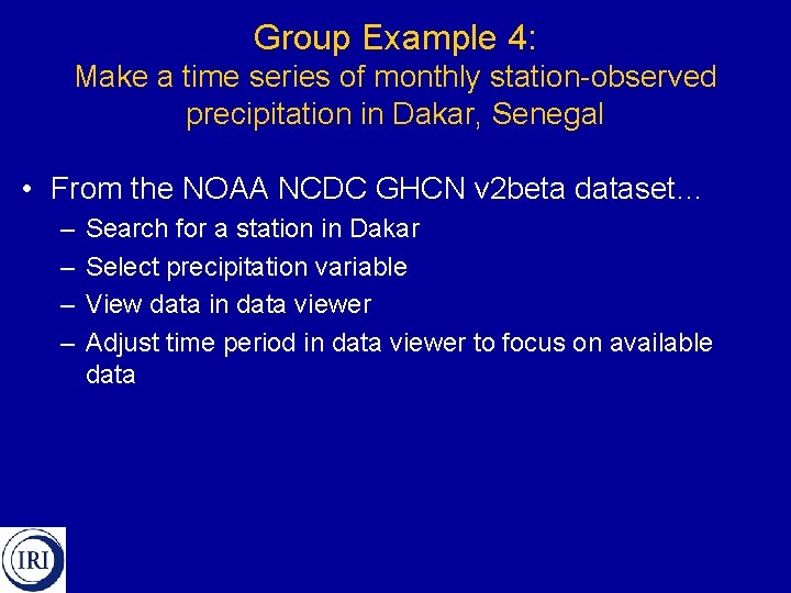
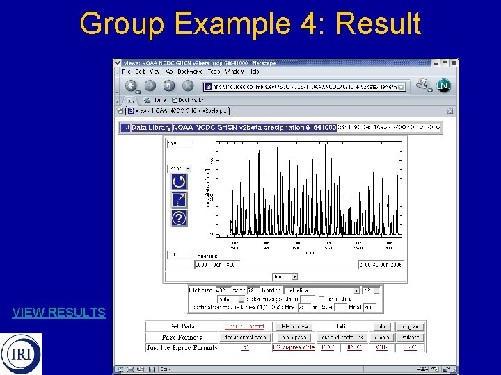
Group Example 4: Make a time series of monthly station-observed precipitation in Dakar, Senegal • From the NOAA NCDC GHCN v 2 beta dataset… – – Search for a station in Dakar Select precipitation variable View data in data viewer Adjust time period in data viewer to focus on available data

Group Example 4: Result VIEW RESULTS

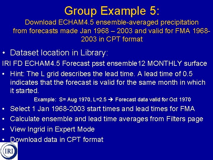
Group Example 5: Download ECHAM 4. 5 ensemble-averaged precipitation from forecasts made Jan 1968 – 2003 and valid for FMA 19682003 in CPT format • Dataset location in Library: IRI FD ECHAM 4. 5 Forecast psst ensemble 12 MONTHLY surface • Hint: The L grid describes the lead time. A lead time of 0. 5 indicates that the forecast is valid for the same month in which it started. Example: S= Aug 1970, L=2. 5 Forecast data valid for Oct 1970 • • Select 1 Jan 1968 -2003 start times and lead times for FMA Calculate ensemble and lead time averages from Filters page View Ingrid in Expert Mode Download data in CPT format

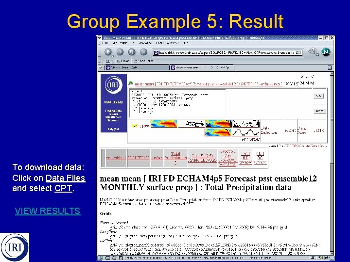
Group Example 5: Result To download data: Click on Data Files and select CPT. VIEW RESULTS

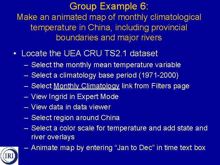
Group Example 6: Make an animated map of monthly climatological temperature in China, including provincial boundaries and major rivers • Locate the UEA CRU TS 2. 1 dataset – – – – Select the monthly mean temperature variable Select a climatology base period (1971 -2000) Select Monthly Climatology link from Filters page View Ingrid in Expert Mode View data in data viewer Select region around China Select a color scale for temperature and add state and river overlays – Animate map by entering “Jan to Dec” in time text box

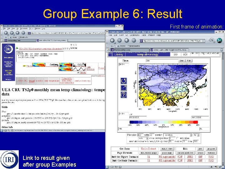
Group Example 6: Result First frame of animation: Link to result given after group Examples

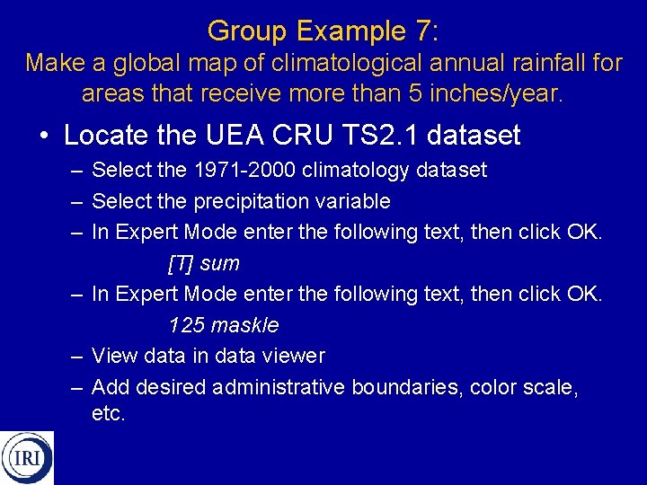
Group Example 7: Make a global map of climatological annual rainfall for areas that receive more than 5 inches/year. • Locate the UEA CRU TS 2. 1 dataset – Select the 1971 -2000 climatology dataset – Select the precipitation variable – In Expert Mode enter the following text, then click OK. [T] sum – In Expert Mode enter the following text, then click OK. 125 maskle – View data in data viewer – Add desired administrative boundaries, color scale, etc.

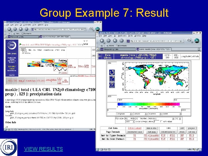
Group Example 7: Result VIEW RESULTS

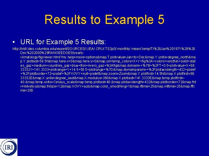
Results to Example 5 • URL for Example 5 Results: http: //iridl. ldeo. columbia. edu/expert/SOURCES/. UEA/. CRU/. TS 2 p 0/. monthly/. mean/. temp/T/%28 Jan%201971%29%28 Dec%202000%29 RANGEEDGES/yearlyclimatology/figviewer. html? my. help=more+options&map. T. plotvalue=Jan+to+Dec&map. Y. units=degree_north&ma p. Y. plotlast=58. 5 N&map. here. x=0&map. here. y=0&map. url=temp_colors+X+Y+fig%3 A+colors+verythin+solid+stat es_gaz+medium+countries_gaz+blue+thin+rivers_gaz+%3 Afig&map. domain=+%7 B+%2 FT+0. 5+plotvalue+X+68. 333321+141. 3333+plotrange+Y+14. 5+58. 5+plotrange+%7 D&map. domainparam=+%2 Fplotaxislength+432+psdef +%2 Fplotborder+72+psdef+%2 FXOVY+null+psdef&map. zoom=Zoom&map. Y. plotfirst=14. 5 N&map. X. plotfirst=68. 33332 E&map. X. units=degree_east&map. X. modulus=360&map. X. plotlast=141. 3333 E&map. temp. plotfirst=40. &map. temp. units=Celsius_scale&map. temp. plotlast=40. &map. plotaxislength=432&map. plotborder=72&map. fnt =Helvetica&map. fntsze=12&map. XOVY=auto&map. color_smoothing=1&map. iftime=25&map. mftime=25&map. ffti me=200

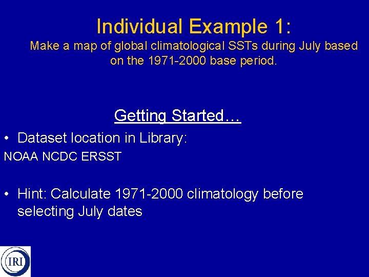
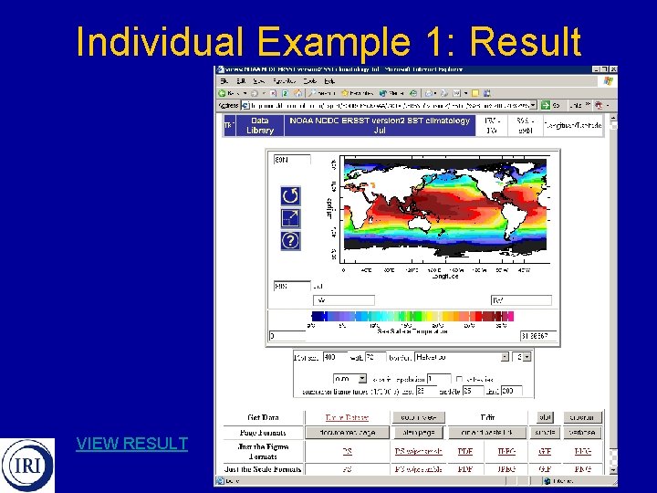
Individual Example 1: Make a map of global climatological SSTs during July based on the 1971 -2000 base period. Getting Started… • Dataset location in Library: NOAA NCDC ERSST • Hint: Calculate 1971 -2000 climatology before selecting July dates

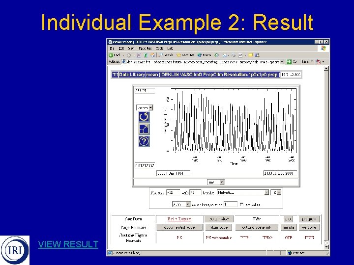
Individual Example 2: Create a time series of monthly precipitation which has been spatially averaged over the Sahel for 1951 -2000 Getting Started… • Dataset location in Library: DEKLIM VASClim. O Prcp. Clim Res-1 x 1 • Approx Sahel region: 7º-22ºN, 17ºW-28ºE

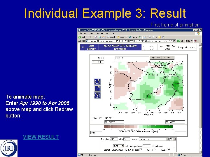
Individual Example 3: Make an animated map of April soil moisture anomalies in Afghanistan during 1990 -2006 Getting Started… • Dataset location in Library: NOAA NCEP CPC GMSM • Hint: Calculate anomalies before selecting April dates

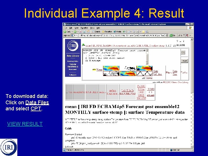
Individual Example 4: Download ECHAM 4. 5 ensemble-averaged surface temperature from forecasts made 1 May 1968 – 2003 and valid for JAS 1968 -2003 in CPT format Getting Started… • Dataset location in Library: IRI FD ECHAM 4. 5 Forecast psst ensemble 12 MONTHLY surface

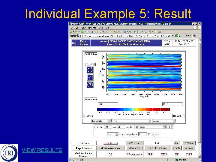
Individual Example 5: Create a time-longitude plot of weekly SSTA in the Tropical Pacific for Jan 1982 -Dec 2005. Use data from 5ºS-5ºN. Getting Started… • Hint: There are two datasets that include weekly seaair interface data. Use the one that has an ssta variable so you do not have to calculate it yourself.

Individual Example 1: Result VIEW RESULT

Individual Example 2: Result VIEW RESULT

Individual Example 3: Result First frame of animation: To animate map: Enter Apr 1990 to Apr 2006 above map and click Redraw button. VIEW RESULT

Individual Example 4: Result To download data: Click on Data Files and select CPT. VIEW RESULT

Individual Example 5: Result VIEW RESULTS