gro Tutorial 1 Eric Klavins Install gro Go

gro Tutorial 1 Eric Klavins

Install gro Go to http: //depts. washington. edu/soslab/gro/download. php and download the latest version of gro to your computer. Follow the installation guide at http: //depts. washington. edu/soslab/gro/docview. html Note that wherever you put gro, you need to have the include file and the examples file in the same directory as the gro executable.

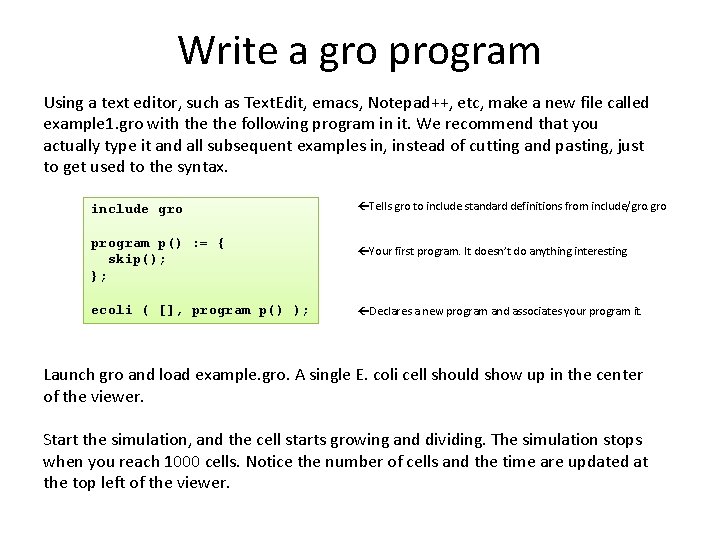
Write a gro program Using a text editor, such as Text. Edit, emacs, Notepad++, etc, make a new file called example 1. gro with the following program in it. We recommend that you actually type it and all subsequent examples in, instead of cutting and pasting, just to get used to the syntax. include gro program p() : = { skip(); }; ecoli ( [], program p() ); Tells gro to include standard definitions from include/gro. gro Your first program. It doesn’t do anything interesting. Declares a new program and associates your program it. Launch gro and load example. gro. A single E. coli cell should show up in the center of the viewer. Start the simulation, and the cell starts growing and dividing. The simulation stops when you reach 1000 cells. Notice the number of cells and the time are updated at the top left of the viewer.

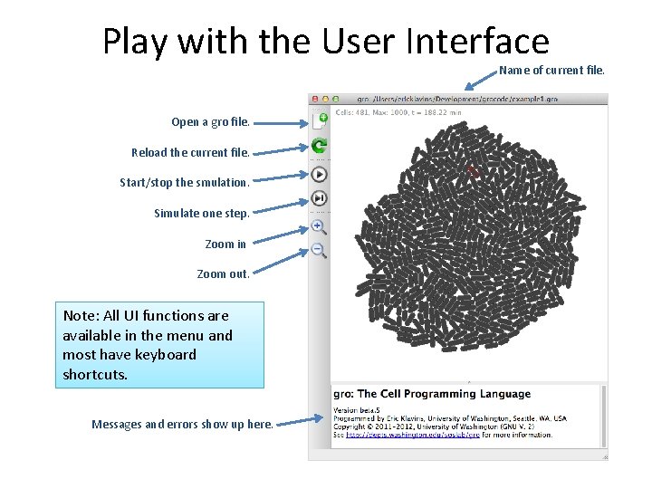
Play with the User Interface Name of current file. Open a gro file. Reload the current file. Start/stop the smulation. Simulate one step. Zoom in Zoom out. Note: All UI functions are available in the menu and most have keyboard shortcuts. Messages and errors show up here.

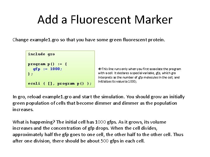
Add a Fluorescent Marker Change example 1. gro so that you have some green fluorescent protein. include gro program p() : = { gfp : = 1000; }; ecoli ( [], program p() ); This line runs only when you first associate the program with a cell. It declares a special variable, gfp, which gro interprets as the number of gfp molecules in the cell, and initializes its value to 1000; In gro, reload example 1. gro and start the simulation. You should grow an initially green population of cells that become dimmer and dimmer as the population increases. What is happening? The initial cell has 1000 gfps. As it grows, its volume increases and the concentration of gfp drops. When the cell divides, approximately half the gfp goes to one cell, the other half to the other cell. Thus after one division, there should be about 500 gfps in each cell.

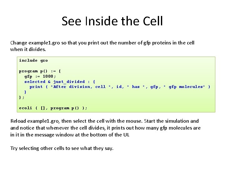
See Inside the Cell Change example 1. gro so that you print out the number of gfp proteins in the cell when it divides. include gro program p() : = { gfp : = 1000; selected & just_divided : { print ( "After division, cell ", id, " has ", gfp, " gfp molecules" ) } }; ecoli ( [], program p() ); Reload example 1. gro, then select the cell with the mouse. Start the simulation and notice that whenever the cell divides, it prints out how many gfp molecules are in it in the message window at the bottom of the UI. Try selecting other cells to see what they say.

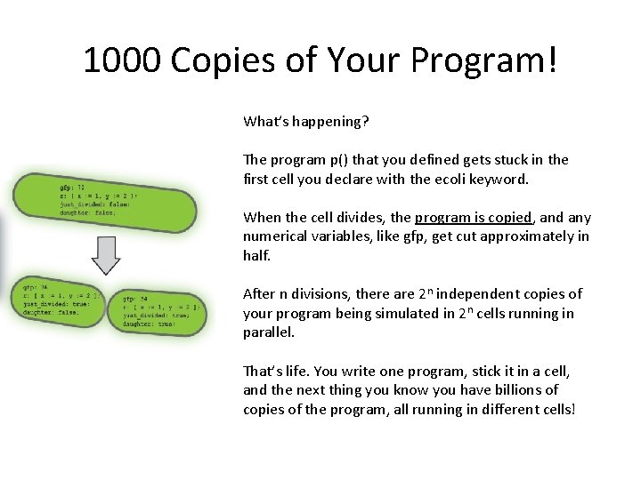
1000 Copies of Your Program! What’s happening? The program p() that you defined gets stuck in the first cell you declare with the ecoli keyword. When the cell divides, the program is copied, and any numerical variables, like gfp, get cut approximately in half. After n divisions, there are 2 n independent copies of your program being simulated in 2 n cells running in parallel. That’s life. You write one program, stick it in a cell, and the next thing you know you have billions of copies of the program, all running in different cells!

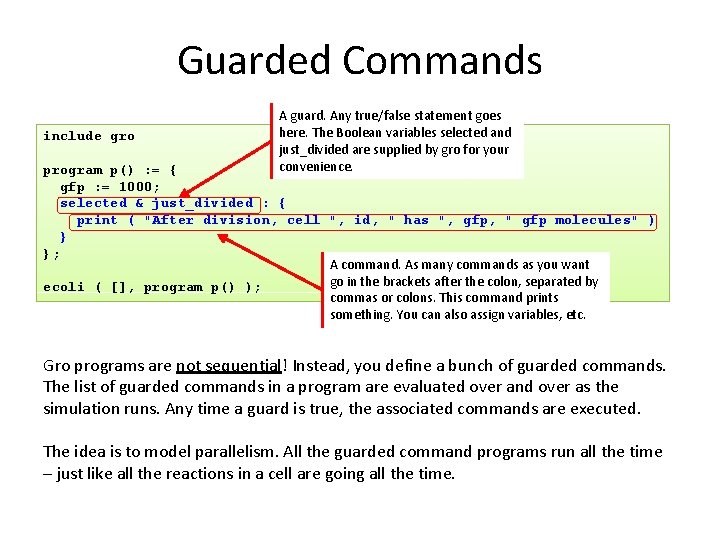
Guarded Commands include gro A guard. Any true/false statement goes here. The Boolean variables selected and just_divided are supplied by gro for your convenience. program p() : = { gfp : = 1000; selected & just_divided : { print ( "After division, cell ", id, " has ", gfp, " gfp molecules" ) } }; A command. As many commands as you want go in the brackets after the colon, separated by ecoli ( [], program p() ); commas or colons. This command prints something. You can also assign variables, etc. Gro programs are not sequential! Instead, you define a bunch of guarded commands. The list of guarded commands in a program are evaluated over and over as the simulation runs. Any time a guard is true, the associated commands are executed. The idea is to model parallelism. All the guarded command programs run all the time – just like all the reactions in a cell are going all the time.

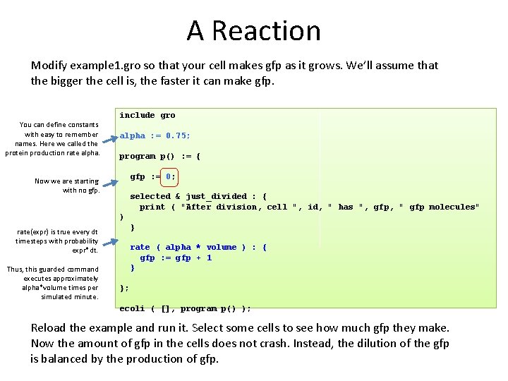
A Reaction Modify example 1. gro so that your cell makes gfp as it grows. We’ll assume that the bigger the cell is, the faster it can make gfp. You can define constants with easy to remember names. Here we called the protein production rate alpha. include gro alpha : = 0. 75; program p() : = { gfp : = 0; Now we are starting with no gfp. selected & just_divided : { print ( "After division, cell ", id, " has ", gfp, " gfp molecules" ) } rate(expr) is true every dt timesteps with probability expr*dt. Thus, this guarded command executes approximately alpha*volume times per simulated minute. rate ( alpha * volume ) : { gfp : = gfp + 1 } }; ecoli ( [], program p() ); Reload the example and run it. Select some cells to see how much gfp they make. Now the amount of gfp in the cells does not crash. Instead, the dilution of the gfp is balanced by the production of gfp.

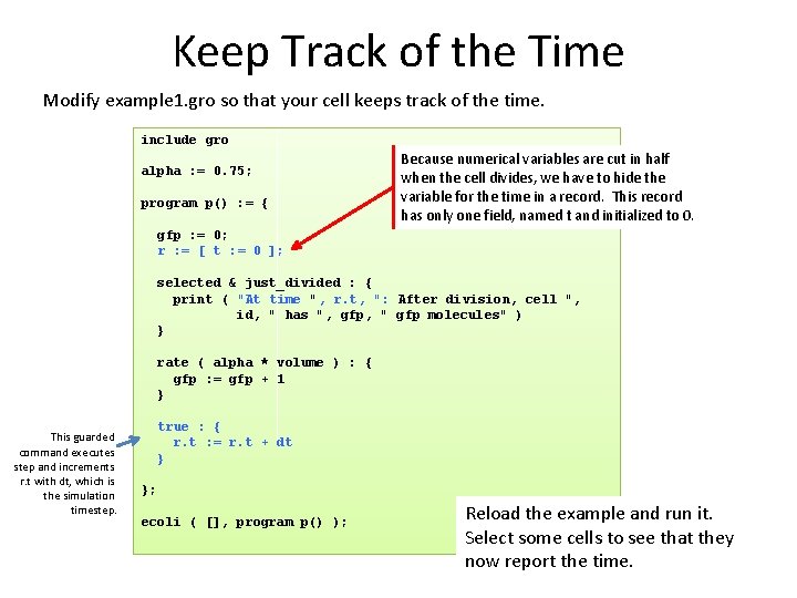
Keep Track of the Time Modify example 1. gro so that your cell keeps track of the time. include gro alpha : = 0. 75; program p() : = { Because numerical variables are cut in half when the cell divides, we have to hide the variable for the time in a record. This record has only one field, named t and initialized to 0. gfp : = 0; r : = [ t : = 0 ]; selected & just_divided : { print ( "At time ", r. t, ": After division, cell ", id, " has ", gfp, " gfp molecules" ) } rate ( alpha * volume ) : { gfp : = gfp + 1 } This guarded command executes step and increments r. t with dt, which is the simulation timestep. true : { r. t : = r. t + dt } }; ecoli ( [], program p() ); Reload the example and run it. Select some cells to see that they now report the time.

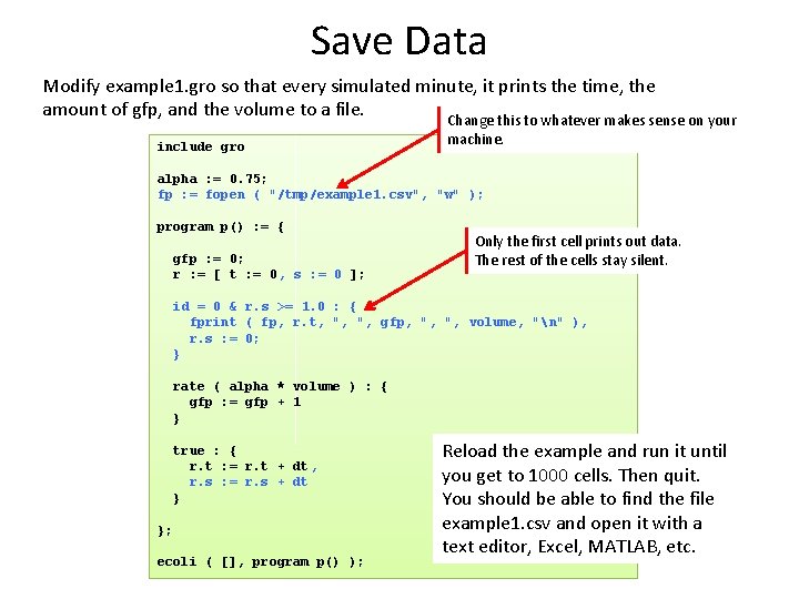
Save Data Modify example 1. gro so that every simulated minute, it prints the time, the amount of gfp, and the volume to a file. Change this to whatever makes sense on your include gro machine. alpha : = 0. 75; fp : = fopen ( "/tmp/example 1. csv", "w" ); program p() : = { gfp : = 0; r : = [ t : = 0, s : = 0 ]; Only the first cell prints out data. The rest of the cells stay silent. id = 0 & r. s >= 1. 0 : { fprint ( fp, r. t, ", ", gfp, ", ", volume, "n" ), r. s : = 0; } rate ( alpha * volume ) : { gfp : = gfp + 1 } true : { r. t : = r. t + dt, r. s : = r. s + dt } }; ecoli ( [], program p() ); Reload the example and run it until you get to 1000 cells. Then quit. You should be able to find the file example 1. csv and open it with a text editor, Excel, MATLAB, etc.

View the Data in Mathematica In Mathematica, you can plot the data as follows.

Overlay an ODE Model c[t] is the concentration of gfp. 0. 75 is alpha from your example 1. gro This number is the growth rate, which you can find in include/gro.

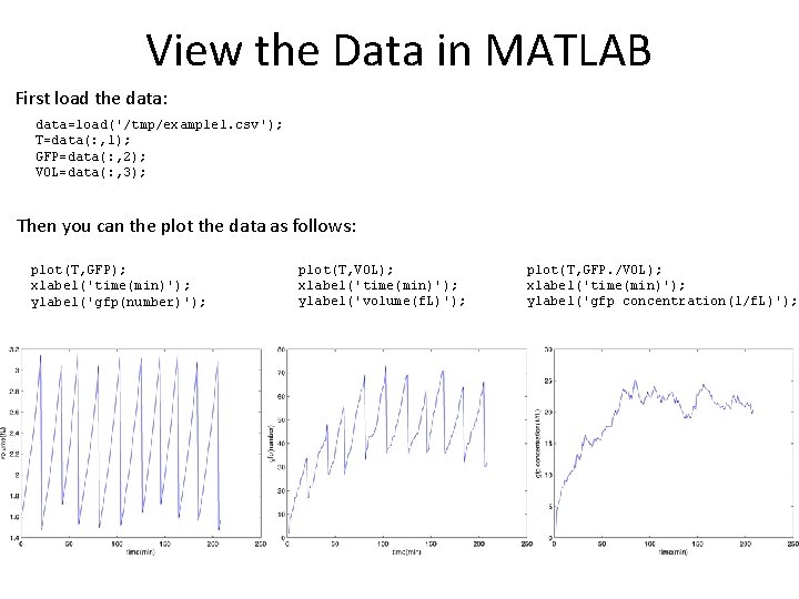
View the Data in MATLAB First load the data: data=load('/tmp/example 1. csv'); T=data(: , 1); GFP=data(: , 2); VOL=data(: , 3); Then you can the plot the data as follows: plot(T, GFP); xlabel('time(min)'); ylabel('gfp(number)'); plot(T, VOL); xlabel('time(min)'); ylabel('volume(f. L)'); plot(T, GFP. /VOL); xlabel('time(min)'); ylabel('gfp concentration(1/f. L)');

Overlay an ODE Model Make a new file, f. m function [ dc ] = f( t, c ) dc = 0. 75 - 0. 0346574*c end 0. 75 is alpha from your example 1. gro c is the concentration of gfp. This number is the growth rate, which you can find in include/gro. Then use ode 45 to solve your differential equation, and overlay the plots: c 0 = 0; tf = max(T); [T 2, C] = ode 45(@f, [t 0, tf], c 0) ; hold on; plot(T 2, C, 'Color', [255 127 0]/255); hold off; xlabel('time(min)'); ylabel('gfp concentration(1/f. L)');

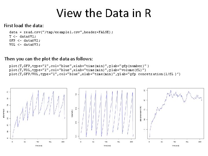
View the Data in R First load the data: data = read. csv("/tmp/example 1. csv", header=FALSE); T <- data$V 1; GFP <- data$V 2; VOL <- data$V 3; Then you can the plot the data as follows: plot(T, GFP, type="l", col="blue", xlab="time(min)", ylab="gfp(number)" ) plot(T, VOL, type="l", col="blue", xlab="time(min)", ylab="volume(f. L)") plot(T, GFP/VOL, type="l", col="blue", xlab="time(min)", ylab="gfp concetration(1/f. L )”)

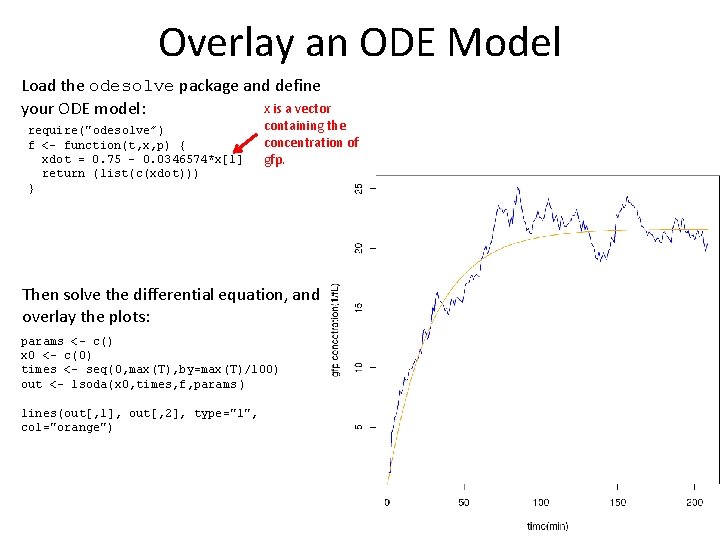
Overlay an ODE Model Load the odesolve package and define x is a vector your ODE model: require("odesolve”) f <- function(t, x, p) { xdot = 0. 75 - 0. 0346574*x[1] return (list(c(xdot))) } containing the concentration of gfp. Then solve the differential equation, and overlay the plots: params <- c() x 0 <- c(0) times <- seq(0, max(T), by=max(T)/100) out <- lsoda(x 0, times, f, params ) lines(out[, 1], out[, 2], type="l", col="orange")