Greenhouse Gas Emissions Global Climate Models and California
Greenhouse Gas Emissions, Global Climate Models, and California Climate Change Impacts 1
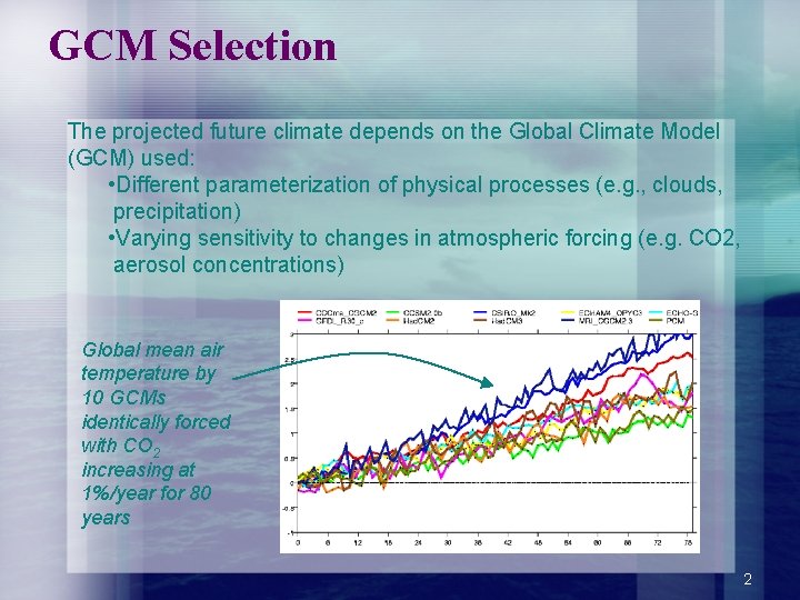
GCM Selection The projected future climate depends on the Global Climate Model (GCM) used: • Different parameterization of physical processes (e. g. , clouds, precipitation) • Varying sensitivity to changes in atmospheric forcing (e. g. CO 2, aerosol concentrations) Global mean air temperature by 10 GCMs identically forced with CO 2 increasing at 1%/year for 80 years 2
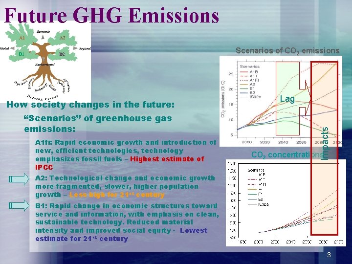
Future GHG Emissions Scenarios of CO 2 emissions “Scenarios” of greenhouse gas emissions: A 1 fi: Rapid economic growth and introduction of new, efficient technologies, technology emphasizes fossil fuels – Highest estimate of IPCC Lag Impacts How society changes in the future: CO 2 concentrations A 2: Technological change and economic growth more fragmented, slower, higher population growth – Less high for 21 st century B 1: Rapid change in economic structures toward service and information, with emphasis on clean, sustainable technology. Reduced material intensity and improved social equity - Lowest estimate for 21 st century 3

GCM Selection – Model Characteristics GFDL 2. 1 – Geophysical Fluid Dynamics Lab, resolution about 2. 0 x 2. 5 degrees (latitude x longitude) PCM – National Center for Atmospheric Research/Dept. of Energy Parallel Climate Model, resolution about 2. 8 degrees Model Characteristics: • Both are Coupled Atmosphere-Ocean-Land models • Neither uses flux adjustments: can simulate stable climate without adjustments • Both are state-of-the-art • Participating in IPCC AR 4 simulations archived at PCMDI, archiving daily data • realistic simulation El Niño SST anomalies – important for CA climate 4

GCM Selection – Sensitivity Difference between all GCMs Average Annual T change over CA Difference between all GCMs B 1 Emission Scenario A 2 Emission Scenario At end of 21 st Century: GFDL slightly drier PCM slightly wetter 1ºC PCM 2ºC GFDL Difference Between GCMs 3ºC PCM 4ºC 5ºC GFDL Difference Between GCMs Difference Between B 1 and A 2 5
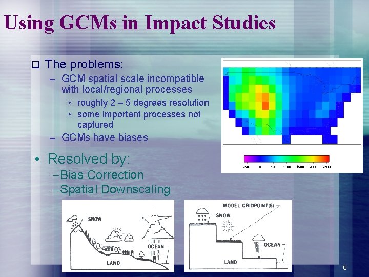
Using GCMs in Impact Studies q The problems: – GCM spatial scale incompatible with local/regional processes • roughly 2 – 5 degrees resolution • some important processes not captured – GCMs have biases • Resolved by: -Bias Correction -Spatial Downscaling 6
Bias Correction Effects q Mean and variability of observed data are reproduced for historical period q Temperature trends into future in GCM output are preserved q Relative changes in mean and variance in future period GCM output are preserved, mapped onto observed variance 7
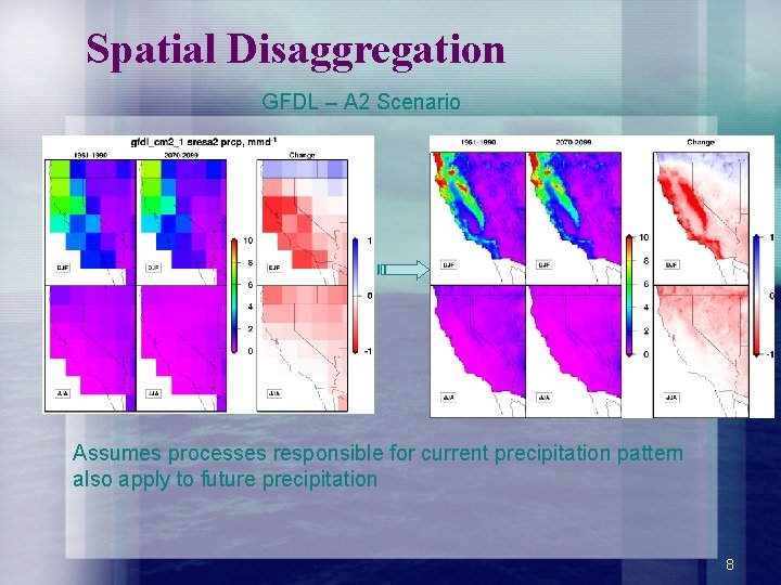
Spatial Disaggregation GFDL – A 2 Scenario Assumes processes responsible for current precipitation pattern also apply to future precipitation 8
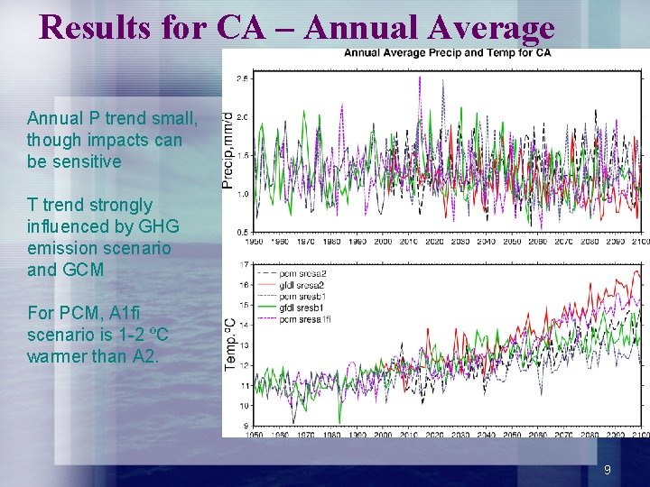
Results for CA – Annual Average Annual P trend small, though impacts can be sensitive T trend strongly influenced by GHG emission scenario and GCM For PCM, A 1 fi scenario is 1 -2 ºC warmer than A 2. 9
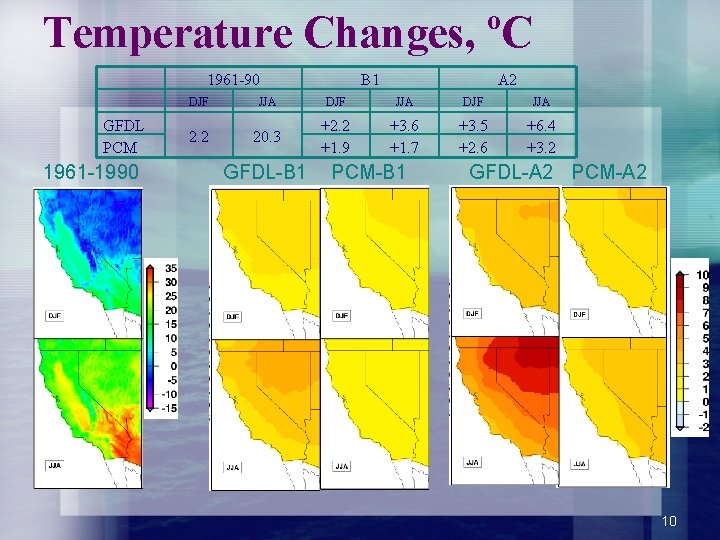
Temperature Changes, ºC 1961 -90 GFDL PCM 1961 -1990 B 1 A 2 DJF JJA 2. 2 20. 3 +2. 2 +1. 9 +3. 6 +1. 7 +3. 5 +2. 6 +6. 4 +3. 2 GFDL-B 1 PCM-B 1 GFDL-A 2 PCM-A 2 10
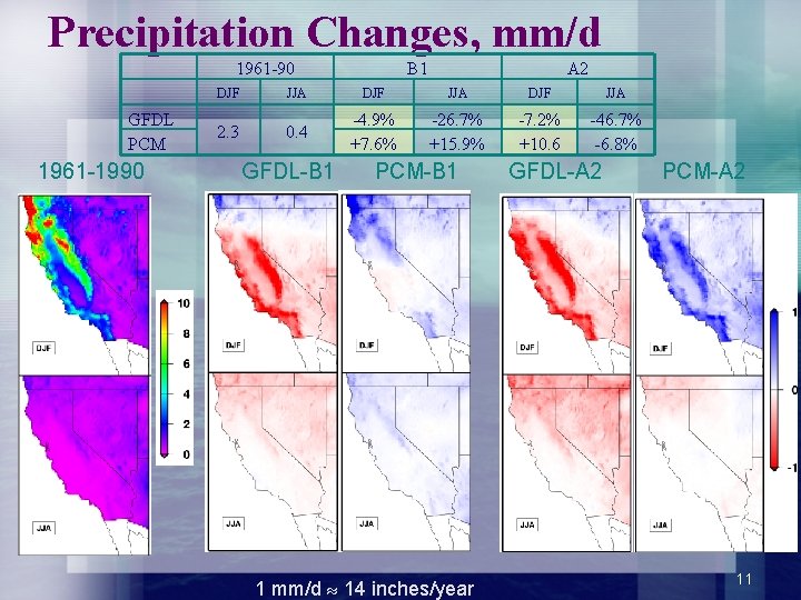
Precipitation Changes, mm/d 1961 -90 GFDL PCM 1961 -1990 B 1 A 2 DJF JJA 2. 3 0. 4 -4. 9% +7. 6% -26. 7% +15. 9% -7. 2% +10. 6 -46. 7% -6. 8% GFDL-B 1 PCM-B 1 1 mm/d 14 inches/year GFDL-A 2 PCM-A 2 11

Derived data for impact modelers Downscaled GCM climate and derived meteorology • precipitation • temperature • humidity • radiation Hydrologic model simulations for specific river basins, have produced: • streamflow • snowpack • snowmelt timing • soil moisture 12
- Slides: 12