Greedy Technique Greedy Technique Constructs a solution to

Greedy Technique

Greedy Technique Constructs a solution to an optimization problem piece by piece through a sequence of choices that are: • feasible, i. e. satisfying the constraints Defined by an objective function and a set of constraints • locally optimal (with respect to some neighborhood definition) • greedy (in terms of some measure), and irrevocable For some problems, it yields a globally optimal solution for every instance. For most, does not but can be useful for fast approximations. We are mostly interested in the former case in this class.

Applications of the Greedy Strategy • Optimal solutions: – – – change making for “normal” coin denominations minimum spanning tree (MST) single-source shortest paths simple scheduling problems Huffman codes • Approximations/heuristics: – traveling salesman problem (TSP) – knapsack problem – other combinatorial optimization problems

Minimum Spanning Tree (MST) • Spanning tree of a connected graph G: a connected acyclic subgraph of G that includes all of G’s vertices • Minimum spanning tree of a weighted, connected graph G: a spanning tree of G of the minimum total weight Example: 6 6 c a a 1 4 4 c c a 1 1 2 2 b 3 d

Prim’s MST algorithm • Start with tree T 1 consisting of one (any) vertex and “grow” tree one vertex at a time to produce MST through a series of expanding subtrees T 1, T 2, …, Tn • On each iteration, construct Ti+1 from Ti by adding vertex not in Ti that is closest to those already in Ti (this is a “greedy” step!) • Stop when all vertices are included

Example 4 a b 4 b 3 d 1 6 2 b b c a 1 6 b 3 d 1 6 2 4 c a 2 d c a 1 6 2 3 4 c a 1 6 2 4 c 3 d

Notes about Prim’s algorithm • Efficiency – O(n 2) for weight matrix representation of graph and array implementation of priority queue – O(m log n) for adjacency lists representation of graph with n vertices and m edges and min-heap implementation of the priority queue

Another greedy algorithm for MST: Kruskal’s • Sort the edges in non-decreasing order of lengths • “Grow” tree one edge at a time to produce MST through a series of expanding forests F 1, F 2, …, Fn 1 • On each iteration, add the next edge on the sorted list unless this would create a cycle. (If it would, skip the edge. )

Example 4 4 c a a 1 6 c 2 d 3 4 b a 3 3 a 2 d d c 1 6 2 b b c 1 6 d 3 c a 1 6 2 b c a 1 6 2 4 1 2 b 3 d

Notes about Kruskal’s algorithm • Algorithm looks easier than Prim’s but is harder to implement (checking for cycles!) • Cycle checking: a cycle is created if added edge connects vertices in the same connected component • Runs in O(m log m) time, with m = |E|. The time is mostly spent on sorting.

Shortest Path

Single-Source Shortest Paths Given graph (directed or undirected) G = (V, E) with weight function w: E R and a vertex s V, find for all vertices v V the minimum possible weight for path from s to v. We will discuss two general case algorithms: • Dijkstra's (positive edge weights only) • Bellman-Ford (positive end negative edge weights) If all edge weights are equal (let's say 1), the problem is solved by BFS in (V+E) time.

Shortest paths – Dijkstra’s algorithm Single Source Shortest Paths Problem: Given a weighted connected (directed) graph G, find shortest paths from source vertex s to each of the other vertices Dijkstra’s algorithm: Similar to Prim’s MST algorithm, with a different way of computing numerical labels: Among vertices not already in the tree, it finds vertex u with the smallest sum dv + w(v, u) where v is a vertex for which shortest path has been already found on preceding iterations (such vertices form a tree rooted at s) dv is the length of the shortest path from source s to v w(v, u) is the length (weight) of edge from v to u

Dijkstra’s Algorithm - Example 1 10 2 9 3 4 7 5 2 6

Dijkstra’s Algorithm - Example 1 10 2 9 3 0 4 6 7 5 2

Dijkstra’s Algorithm - Example 1 10 10 2 9 3 0 4 6 7 5 5 2

Dijkstra’s Algorithm - Example 1 10 10 2 9 3 0 4 6 7 5 5 2

Dijkstra’s Algorithm - Example 1 8 10 2 14 9 3 0 4 6 7 5 5 2 7

Dijkstra’s Algorithm - Example 1 8 10 2 14 9 3 0 4 6 7 5 5 2 7

Dijkstra’s Algorithm - Example 1 8 10 2 13 9 3 0 4 6 7 5 5 2 7

Dijkstra’s Algorithm - Example 1 8 10 2 13 9 3 0 4 6 7 5 5 2 7

Dijkstra’s Algorithm - Example 1 8 10 2 9 9 3 0 4 6 7 5 5 2 7

Dijkstra’s Algorithm - Example 1 8 10 2 9 9 3 0 4 6 7 5 5 2 7

executed (V) times (E) times in total (V) (1) SSSP-Dijkstra(graph (G, w), vertex s) Initialize. Single. Source(G, s) S Q V[G] while Q 0 do u Extract. Min(Q) S S {u} for u Adj[u] do Relax(u, v, w) Initialize. Single. Source(graph G, vertex s) for v V[G] do d[v] p[v] 0 d[s] 0 Relax(vertex u, vertex v, weight w) if d[v] > d[u] + w(u, v) then d[v] d[u] + w(u, v) p[v] u

Dijkstra’s Algorithm - Complexity

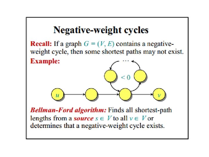
Bellman-Ford Algorithm - negative cycles?

Bellman-Ford Algorithm - Idea The Bellman–Ford algorithm is an algorithm that computes shortest paths from a single source vertex to all of the other vertices in a weighted digraph. [1] It is slower than Dijkstra's algorithm for the same problem, but more versatile, as it is capable of handling graphs in which some of the edge weights are negative numbers.

Bellman-Ford Algorithm - SSSPBellman. Ford SSSP-Bellman. Ford(graph (G, w), vertex s) Initialize. Single. Source(G, s) for i 1 to |V[G] 1| do for (u, v) E[G] do Relax(u, v, w) for (u, v) E[G] do if d[v] > d[u] + w(u, v) then return false return true

Bellman-Ford Algorithm - Example -2 5 6 -3 8 2 7 9 -4 7

Bellman-Ford Algorithm - Example -2 6 5 -3 8 0 2 7 9 7 -4

Bellman-Ford Algorithm - Example -2 6 5 6 -3 8 0 2 7 7 9 7 -4

Bellman-Ford Algorithm - Example -2 6 5 6 -3 8 0 2 7 7 4 9 7 -4 2

Bellman-Ford Algorithm - Example -2 6 5 2 -3 8 0 2 7 7 4 9 7 -4 2

Bellman-Ford Algorithm - Example -2 6 5 2 -3 8 0 2 7 7 4 9 -4 7 -2

Bellman-Ford Algorithm - Complexity executed (V) times (E) = (V E) SSSP-Bellman. Ford(graph (G, w), vertex s) Initialize. Single. Source(G, s) for i 1 to |V[G] 1| do for (u, v) E[G] do Relax(u, v, w) (1) for (u, v) E[G] do if d[v] > d[u] + w(u, v) then return false return true

All Pair shortest path algorithm • -- Warshall’s Algo • -- Floyd’s Algo

Coding Problem Coding: assignment of bit strings to alphabet characters E. g. We can code {a, b, c, d} as {00, 01, 10, 11} or {0, 110, 111} or {0, 01, 101} }. Codewords: bit strings assigned for characters of alphabet Two types of codes: • fixed-length encoding (e. g. , ASCII) • variable-length encoding (e, g. , Morse code) It allows for efficient (online) decoding! 10010110… Prefix-free codes (or prefix-codes): no codeword is a prefix of another codeword

Huffman codes • Any binary tree with edges labeled with 0’s and 1’s yields a prefix-free code of characters assigned to its leaves 0 • Optimal binary tree minimizing the average length of a codeword can be constructed as follows: 0 1 1 1 represents {00, 011, 1} Huffman’s algorithm Initialize n one-node trees with alphabet characters and the tree weights with their frequencies. Repeat the following step n-1 times: join two binary trees with smallest weights into one (as left and right subtrees) and make its weight equal the sum of the weights of the two trees. Mark edges leading to left and right subtrees with 0’s and 1’s, respectively.

Example character A B C D _ frequency 0. 35 0. 1 0. 2 0. 15 codeword 11 100 00 01 101 average bits per character: 2. 25 for fixed-length encoding: 3

Maximum Flow Problem of maximizing the flow of a material through a transportation network (e. g. , pipeline system, communications or transportation networks) Formally represented by a connected weighted digraph with n vertices numbered from 1 to n with the following properties: – contains exactly one vertex with no entering edges, called the source (numbered 1) – contains exactly one vertex with no leaving edges, called the sink (numbered n) – has positive integer weight uij on each directed edge (i. j), called the edge capacity, indicating the upper bound on the amount of the material that can be sent from i to j through this edge

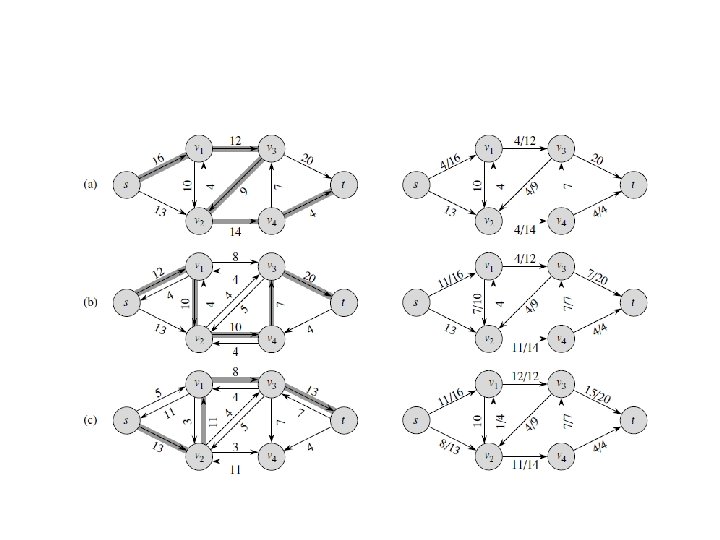
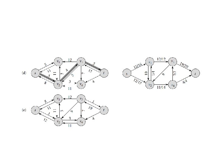
Example of Flow Network 5 4 3 Source 2 1 2 5 3 2 6 Sink 3 1 4

Definition of a Flow A flow is an assignment of real numbers xij to edges (i, j) of a given network that satisfy the following: • flow-conservation requirements The total amount of material entering an intermediate vertex must be equal to the total amount of the material leaving the vertex ∑ xji = ∑ xij for i = 2, 3, …, n-1 j: (j, i) є E j: (i, j) є E • capacity constraints 0 ≤ xij ≤ uij for every edge (i, j) E

Flow value and Maximum Flow Problem Since no material can be lost or added to by going through intermediate vertices of the network, the total amount of the material leaving the source must end up at the sink: ∑ x 1 j = ∑ xjn j: (1, j) є E j: (j, n) є E The value of the flow is defined as the total outflow from the source (= the total inflow into the sink). The maximum flow problem is to find a flow of the largest value (maximum flow) for a given network.

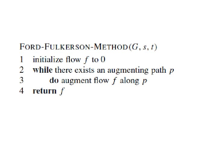
Augmenting Path (Ford-Fulkerson) Method • Start with the zero flow (xij = 0 for every edge) • On each iteration, try to find a flow-augmenting path from source to sink, which a path along which some additional flow can be sent • If a flow-augmenting path is found, adjust the flow along the edges of this path to get a flow of increased value and try again • If no flow-augmenting path is found, the current flow is maximum

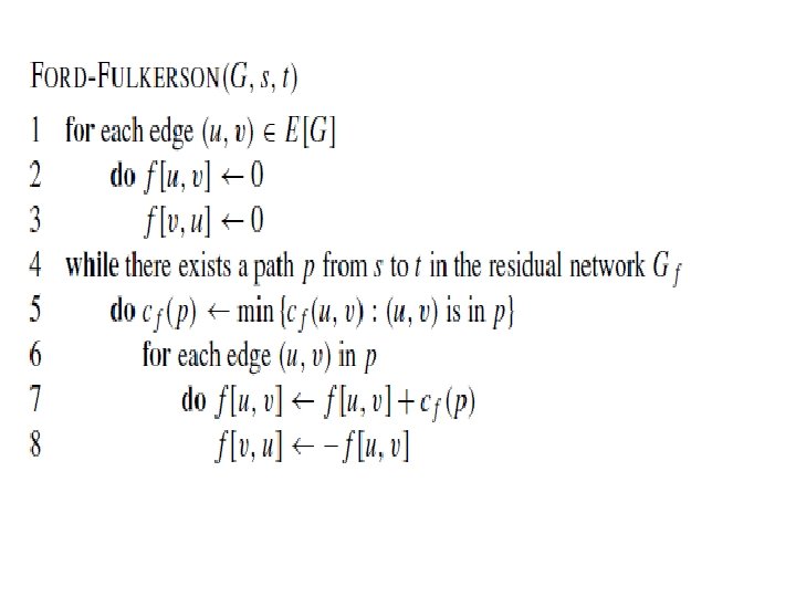
Finding a flow-augmenting path To find a flow-augmenting path for a flow x, consider paths from source to sink in the underlying undirected graph in which any two consecutive vertices i, j are either: – connected by a directed edge (i to j) with some positive unused capacity rij = uij – xij • known as forward edge ( → ) OR – connected by a directed edge (j to i) with positive flow xji • known as backward edge ( ← ) If a flow-augmenting path is found, the current flow can be increased by r units by increasing xij by r on each forward edge and decreasing xji by r on each backward edge, where r = min {rij on all forward edges, xji on all backward edges}

Finding a flow-augmenting path (cont. ) • Assuming the edge capacities are integers, r is a positive integer • On each iteration, the flow value increases by at least 1 • Maximum value is bounded by the sum of the capacities of the edges leaving the source; hence the augmenting-path method has to stop after a finite number of iterations • The final flow is always maximum, its value doesn’t depend on a sequence of augmenting paths used