Greedy Algorithms Lecture 10 Asst Prof Dr lker

Greedy Algorithms Lecture 10 Asst. Prof. Dr. İlker Kocabaş 1

Introduction • A greedy algorithm always makes the choice that looks best at the moment. • That is, it makes a locally optimal choice in the hope that this choice will lead to a globally optimal solution. 2

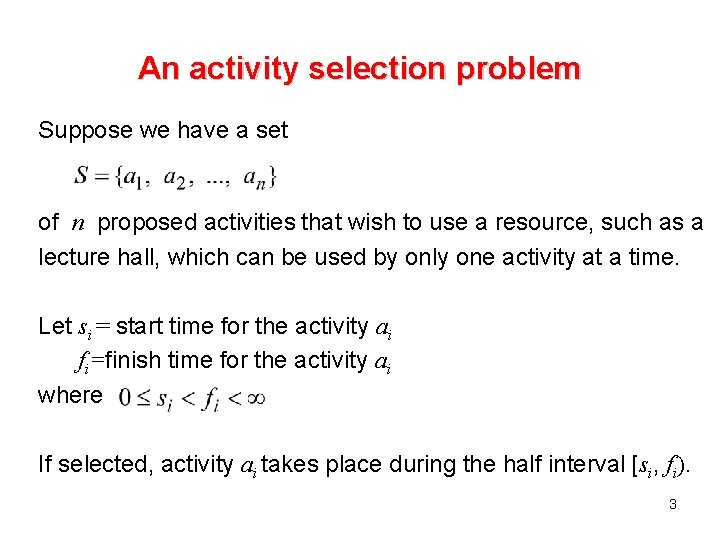
An activity selection problem Suppose we have a set of n proposed activities that wish to use a resource, such as a lecture hall, which can be used by only one activity at a time. Let si = start time for the activity ai fi=finish time for the activity ai where If selected, activity ai takes place during the half interval [si, fi). 3

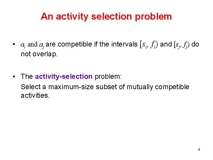
An activity selection problem • ai and aj are competible if the intervals [si, fi) and [sj, fj) do not overlap. • The activity-selection problem: Select a maximum-size subset of mutually competible activities. 4

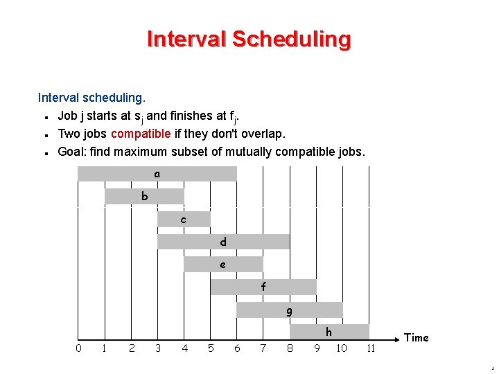
Interval Scheduling Interval scheduling. Job j starts at sj and finishes at fj. Two jobs compatible if they don't overlap. Goal: find maximum subset of mutually compatible jobs. n n n a b c d e f g h 0 1 2 3 4 5 6 7 8 9 10 11 Time 5

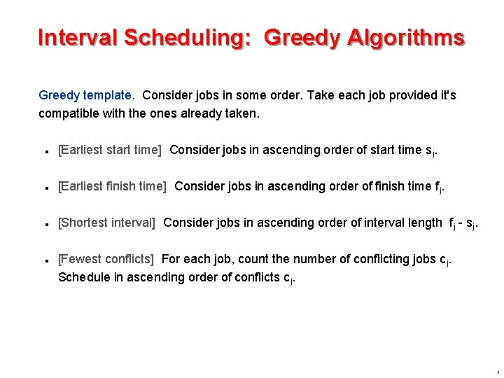
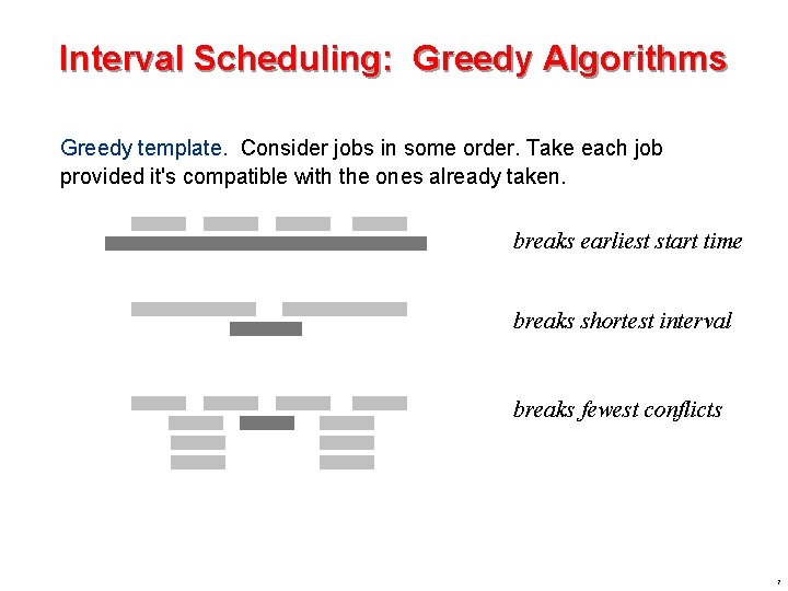
Interval Scheduling: Greedy Algorithms Greedy template. Consider jobs in some order. Take each job provided it's compatible with the ones already taken. n [Earliest start time] Consider jobs in ascending order of start time sj. n [Earliest finish time] Consider jobs in ascending order of finish time fj. n [Shortest interval] Consider jobs in ascending order of interval length fj - sj. n [Fewest conflicts] For each job, count the number of conflicting jobs cj. Schedule in ascending order of conflicts cj. 6

Interval Scheduling: Greedy Algorithms Greedy template. Consider jobs in some order. Take each job provided it's compatible with the ones already taken. breaks earliest start time breaks shortest interval breaks fewest conflicts 7

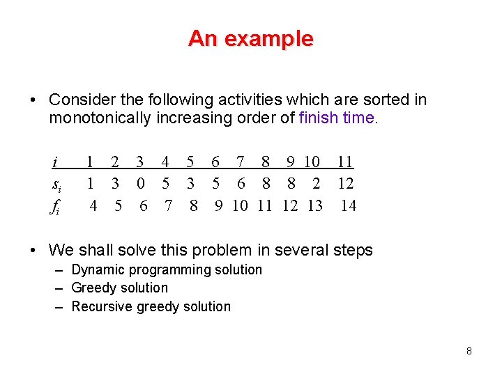
An example • Consider the following activities which are sorted in monotonically increasing order of finish time. i si fi 1 2 3 4 5 6 7 8 9 10 11 1 3 0 5 3 5 6 8 8 2 12 4 5 6 7 8 9 10 11 12 13 14 • We shall solve this problem in several steps – Dynamic programming solution – Greedy solution – Recursive greedy solution 8

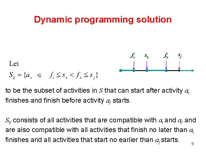
Dynamic programming solution fi sx fx sj to be the subset of activities in S that can start after activity ai finishes and finish before activity aj starts. Sij consists of all activities that are compatible with ai and aj and are also compatible with all activities that finish no later than ai finishes and all activities that start no earlier than aj starts. 9

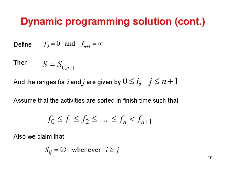
Dynamic programming solution (cont. ) Define Then And the ranges for i and j are given by Assume that the activities are sorted in finish time such that Also we claim that 10

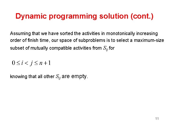
Dynamic programming solution (cont. ) Assuming that we have sorted the activities in monotonically increasing order of finish time, our space of subproblems is to select a maximum-size subset of mutually compatible activities from Sij for knowing that all other Sij are empty. 11

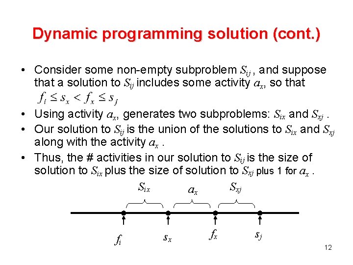
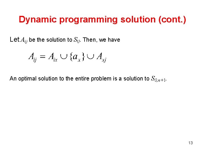
Dynamic programming solution (cont. ) • Consider some non-empty subproblem Sij , and suppose that a solution to Sij includes some activity ax, so that • Using activity ax, generates two subproblems: Six and Sxj. • Our solution to Sij is the union of the solutions to Six and Sxj along with the activity ax. • Thus, the # activities in our solution to Sij is the size of solution to Six plus the size of solution to Sxj plus 1 for ax. Six Sxj ax fi sx fx sj 12

Dynamic programming solution (cont. ) Let Aij be the solution to Sij. Then, we have An optimal solution to the entire problem is a solution to S 0, n+1. 13

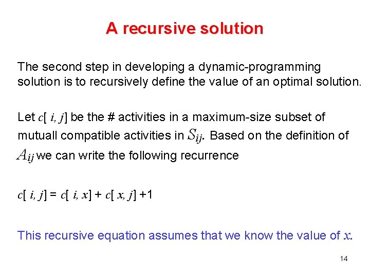
A recursive solution The second step in developing a dynamic-programming solution is to recursively define the value of an optimal solution. Let c[ i, j] be the # activities in a maximum-size subset of mutuall compatible activities in Sij. Based on the definition of Aij we can write the following recurrence c[ i, j] = c[ i, x] + c[ x, j] +1 This recursive equation assumes that we know the value of x. 14

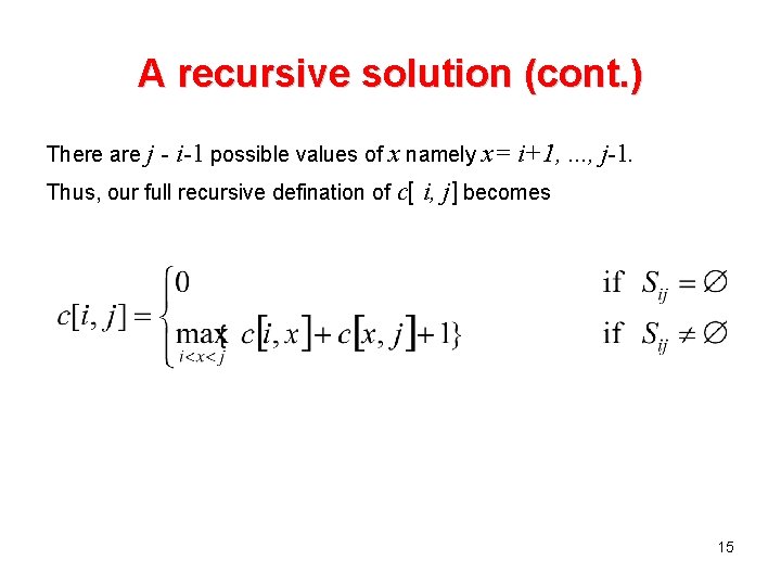
A recursive solution (cont. ) There are j - i-1 possible values of x namely x= i+1, . . . , j-1. Thus, our full recursive defination of c[ i, j] becomes 15

A bottom-up dynamic-programming solution • It is straightforward to write a tabular, bottom-up dynamic-programming algorithm based on the above recurrence 16

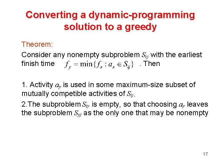
Converting a dynamic-programming solution to a greedy Theorem: Consider any nonempty subproblem Sij with the earliest finish time. Then 1. Activity ay is used in some maximum-size subset of mutually competible activities of Sij. 2. The subproblem Siy is empty, so that choosing ay leaves the subproblem Syj as the only one that may be nonempty 17

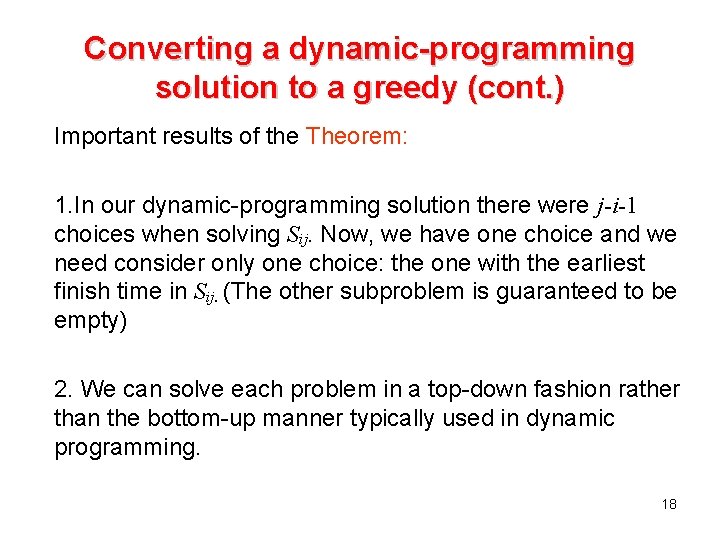
Converting a dynamic-programming solution to a greedy (cont. ) Important results of the Theorem: 1. In our dynamic-programming solution there were j-i-1 choices when solving Sij. Now, we have one choice and we need consider only one choice: the one with the earliest finish time in Sij. (The other subproblem is guaranteed to be empty) 2. We can solve each problem in a top-down fashion rather than the bottom-up manner typically used in dynamic programming. 18

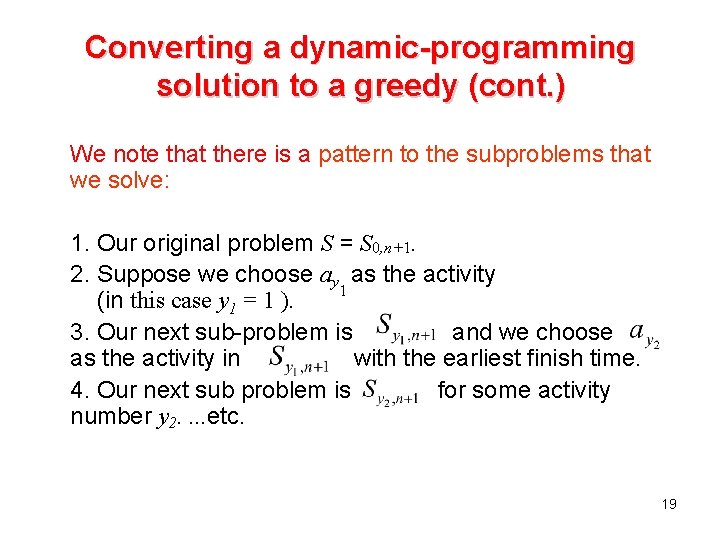
Converting a dynamic-programming solution to a greedy (cont. ) We note that there is a pattern to the subproblems that we solve: 1. Our original problem S = S 0, n+1. 2. Suppose we choose ay as the activity 1 (in this case y 1 = 1 ). 3. Our next sub-problem is and we choose as the activity in with the earliest finish time. 4. Our next sub problem is for some activity number y 2. . etc. 19

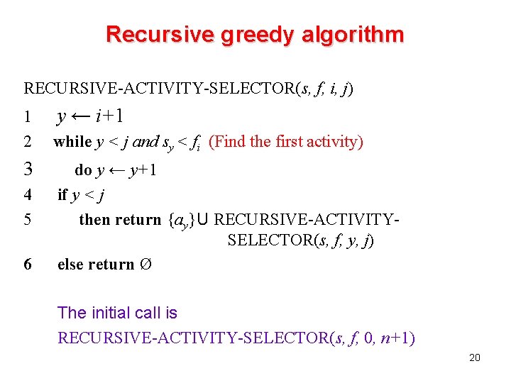
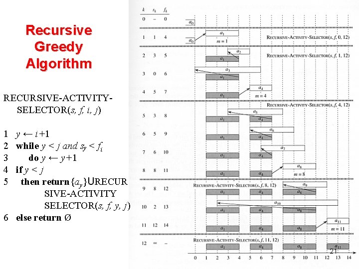
Recursive greedy algorithm RECURSIVE-ACTIVITY-SELECTOR(s, f, i, j) 1 2 3 4 5 6 y ← i+1 while y < j and sy < fi (Find the first activity) do y ← y+1 if y < j then return {ay}U RECURSIVE-ACTIVITYSELECTOR(s, f, y, j) else return Ø The initial call is RECURSIVE-ACTIVITY-SELECTOR(s, f, 0, n+1) 20

Recursive Greedy Algorithm RECURSIVE-ACTIVITYSELECTOR(s, f, i, j) 1 y ← i+1 2 while y < j and sy < fi 3 do y ← y+1 4 if y < j 5 then return{ay}URECUR SIVE-ACTIVITY SELECTOR(s, f, y, j) 6 else return Ø 21

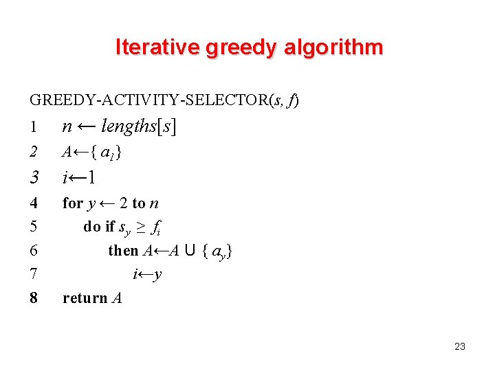
Iterative greedy algorithm 1. 2. 3. We easily can convert our recursive procedure to an iterative one. The following code is an iterative version of the procedure RECURSIVE-ACTIVITY-SELECTOR. It collects selected activities into a set A and returns this set when it is done. 22

Iterative greedy algorithm GREEDY-ACTIVITY-SELECTOR(s, f) 1 2 n ← lengths[s] 3 i← 1 4 5 6 7 8 for y ← 2 to n do if sy ≥ fi then A←A U { ay} i←y return A A←{ a 1} 23

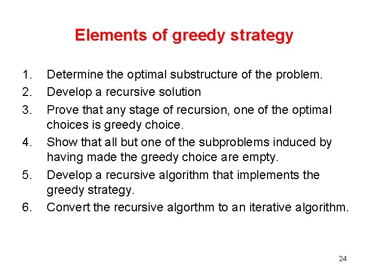
Elements of greedy strategy 1. 2. 3. 4. 5. 6. Determine the optimal substructure of the problem. Develop a recursive solution Prove that any stage of recursion, one of the optimal choices is greedy choice. Show that all but one of the subproblems induced by having made the greedy choice are empty. Develop a recursive algorithm that implements the greedy strategy. Convert the recursive algorthm to an iterative algorithm. 24

Greedy choice property A globally optimal solution can be arrived at by making a locally optimal(greedy) choice. When we are considering which choice to make, we make the choice that looks best in the current problem, without considering results from subproblems 25

Greedy choice property (cont. ) In dynamic programming, we make a choice at each step, but the choice usually depends on the solutions to subproblems. We typically solve dynamic-programming problems in a bottom-up manner. In a greedy algorithm, we make whatever choice seems best at the moment and then solve the subproblem arising after the choice is made. A greedy strategy usually progresses in a top-down fashion, making one greedy choice after another. 26

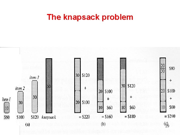
The 0 -1 knapsack problem • • • A thief robbing a store finds n items; the ith item worths vi dollars and weighs wi pounds, where vi and wi are integers. He wants to take as valuable a load as possible, but he can carry at most W pounds in his knapsack for some integer W. Which item should he take? 27

The fractional knapsack problem • The set up is the same, but the thief can take fractions of items, rather than having to make a binary (0 -1) choice for each item. 28

The knapsack problem 29

Huffman codes are widely used and very effective technique for compressing data. We consider the data to be a sequence of charecters. 30

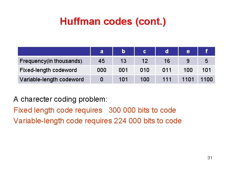
Huffman codes (cont. ) a b c d e f Frequency(in thousands) 45 13 12 16 9 5 Fixed-length codeword 000 001 010 011 100 101 100 111 1100 Variable-length codeword A charecter coding problem: Fixed length code requires 300 000 bits to code Variable-length code requires 224 000 bits to code 31

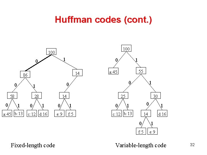
Huffman codes (cont. ) 100 1 0 0 14 86 0 0 28 1 a: 45 b: 13 0 55 a: 45 0 0 1 58 1 25 14 1 c: 12 d: 16 Fixed-length code 1 0 1 e: 9 f: 5 0 30 0 1 c: 12 b: 13 1 14 d: 16 0 1 f: 5 e: 9 Variable-length code 32

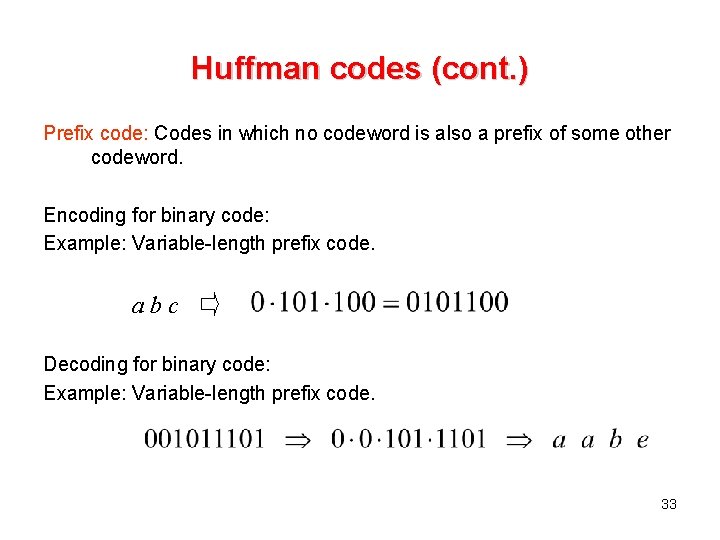
Huffman codes (cont. ) Prefix code: Codes in which no codeword is also a prefix of some other codeword. Encoding for binary code: Example: Variable-length prefix code. abc Decoding for binary code: Example: Variable-length prefix code. 33

Constructing Huffman codes 34

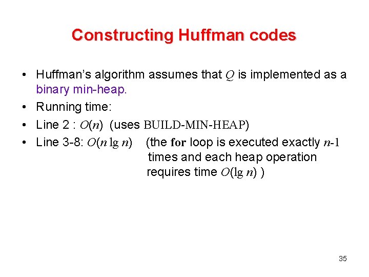
Constructing Huffman codes • Huffman’s algorithm assumes that Q is implemented as a binary min-heap. • Running time: • Line 2 : O(n) (uses BUILD-MIN-HEAP) • Line 3 -8: O(n lg n) (the for loop is executed exactly n-1 times and each heap operation requires time O(lg n) ) 35

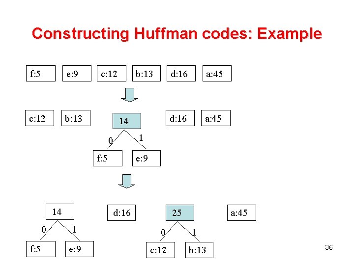
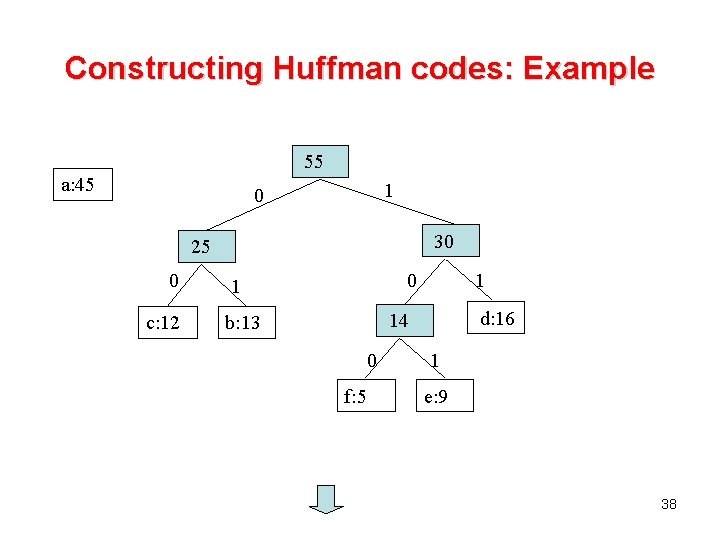
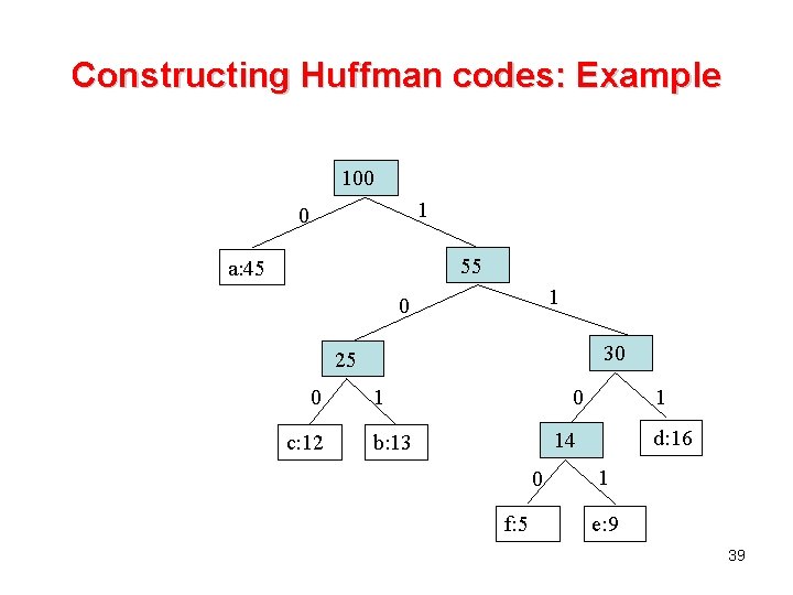
Constructing Huffman codes: Example f: 5 e: 9 c: 12 b: 13 14 f: 5 0 f: 5 e: 9 d: 16 a: 45 e: 9 d: 16 1 a: 45 1 0 14 d: 16 25 0 c: 12 a: 45 1 b: 13 36

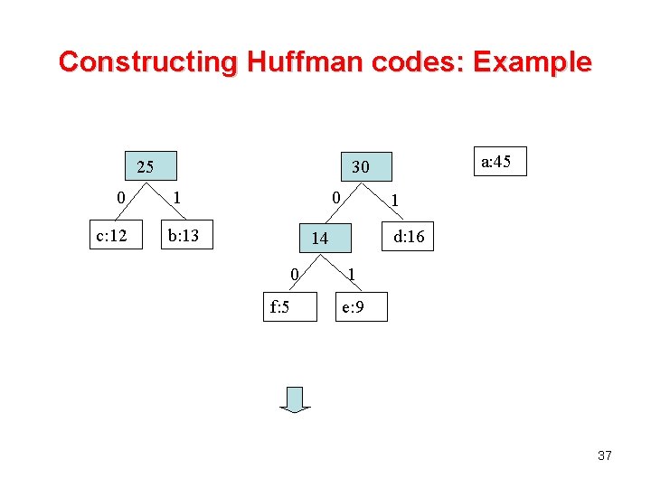
Constructing Huffman codes: Example 25 0 c: 12 a: 45 30 1 0 b: 13 1 d: 16 14 0 f: 5 1 e: 9 37

Constructing Huffman codes: Example 55 a: 45 1 0 30 25 0 c: 12 0 1 1 d: 16 14 b: 13 0 f: 5 1 e: 9 38

Constructing Huffman codes: Example 100 1 0 55 a: 45 1 0 30 25 0 c: 12 1 0 1 d: 16 14 b: 13 0 f: 5 1 e: 9 39

Coin Changing Greed is good. Greed is right. Greed works. Greed clarifies, cuts through, and captures the essence of the evolutionary spirit. - Gordon Gecko (Michael Douglas)

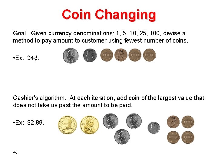
Coin Changing Goal. Given currency denominations: 1, 5, 10, 25, 100, devise a method to pay amount to customer using fewest number of coins. • Ex: 34¢. Cashier's algorithm. At each iteration, add coin of the largest value that does not take us past the amount to be paid. • Ex: $2. 89. 41

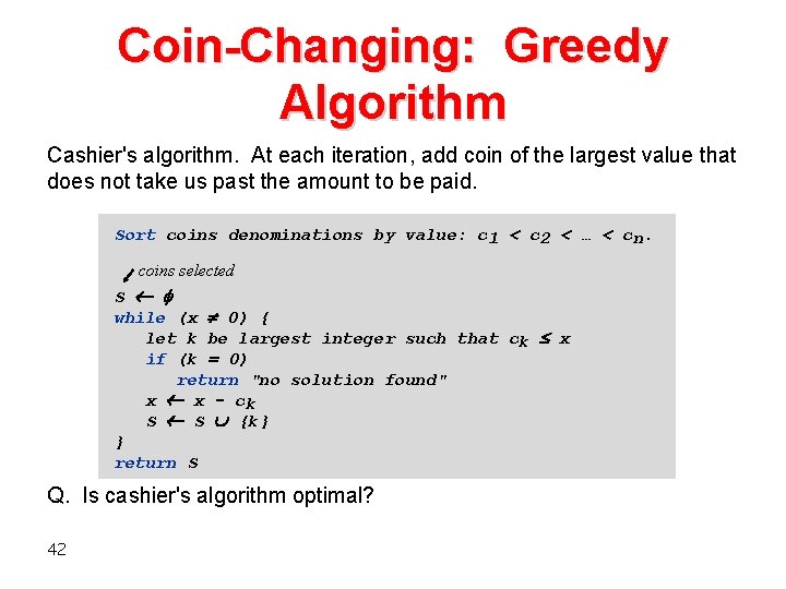
Coin-Changing: Greedy Algorithm Cashier's algorithm. At each iteration, add coin of the largest value that does not take us past the amount to be paid. Sort coins denominations by value: c 1 < c 2 < … < cn. coins selected S while (x 0) { let k be largest integer such that ck x if (k = 0) return "no solution found" x x - ck S S {k} } return S Q. Is cashier's algorithm optimal? 42

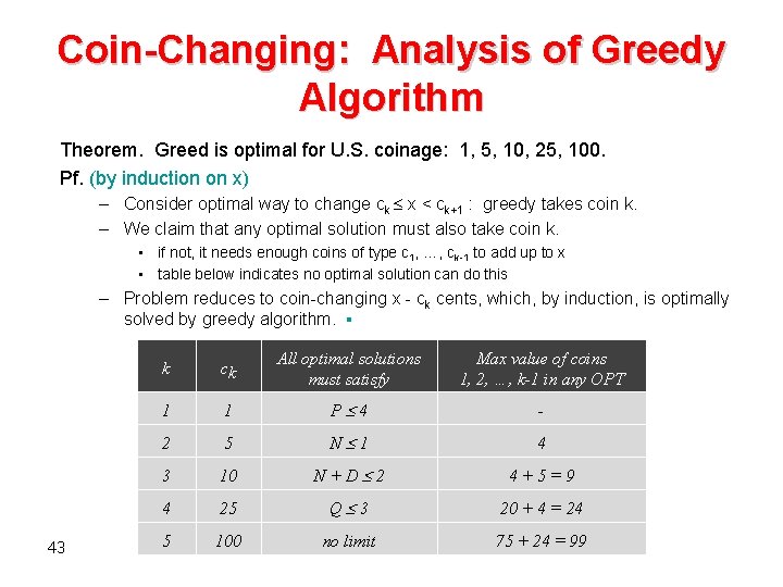
Coin-Changing: Analysis of Greedy Algorithm Theorem. Greed is optimal for U. S. coinage: 1, 5, 10, 25, 100. Pf. (by induction on x) – Consider optimal way to change ck x < ck+1 : greedy takes coin k. – We claim that any optimal solution must also take coin k. • if not, it needs enough coins of type c 1, …, ck-1 to add up to x • table below indicates no optimal solution can do this – Problem reduces to coin-changing x - ck cents, which, by induction, is optimally solved by greedy algorithm. ▪ 43 k ck All optimal solutions must satisfy Max value of coins 1, 2, …, k-1 in any OPT 1 1 P 4 - 2 5 N 1 4 3 10 N+D 2 4+5=9 4 25 Q 3 20 + 4 = 24 5 100 no limit 75 + 24 = 99

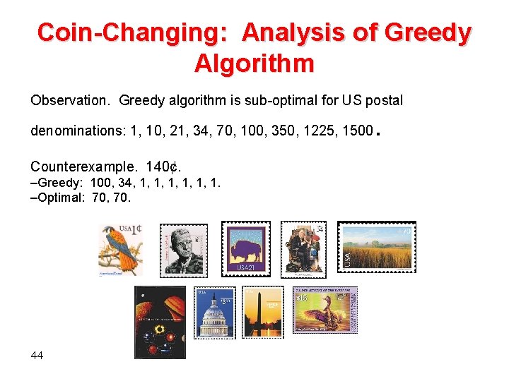
Coin-Changing: Analysis of Greedy Algorithm Observation. Greedy algorithm is sub-optimal for US postal denominations: 1, 10, 21, 34, 70, 100, 350, 1225, 1500 Counterexample. 140¢. –Greedy: 100, 34, 1, 1, 1. –Optimal: 70, 70. 44 .