Greedy Algorithms Interval Scheduling given a set of







- Slides: 109

Greedy Algorithms

Interval Scheduling • given a set of intervals (I 1, I 2, . . . , In) • each interval Ii has a starting time si, a finishing time fi • your task is to find the largest subset of mutually non-overlapping intervals

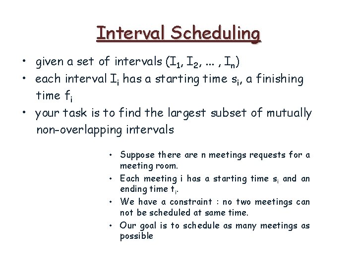
Interval Scheduling • given a set of intervals (I 1, I 2, . . . , In) • each interval Ii has a starting time si, a finishing time fi • your task is to find the largest subset of mutually non-overlapping intervals • Suppose there are n meetings requests for a meeting room. • Each meeting i has a starting time si and an ending time ti. • We have a constraint : no two meetings can not be scheduled at same time. • Our goal is to schedule as many meetings as possible

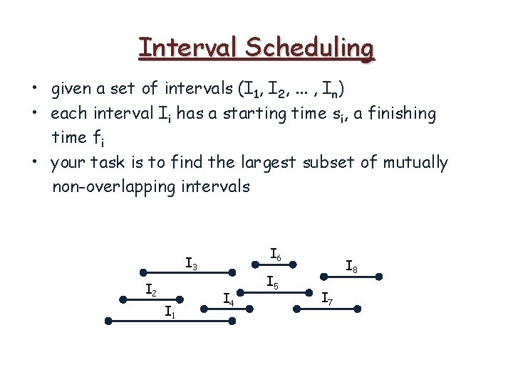
Interval Scheduling • given a set of intervals (I 1, I 2, . . . , In) • each interval Ii has a starting time si, a finishing time fi • your task is to find the largest subset of mutually non-overlapping intervals I 6 I 3 I 2 I 1 I 4 I 5 I 8 I 7

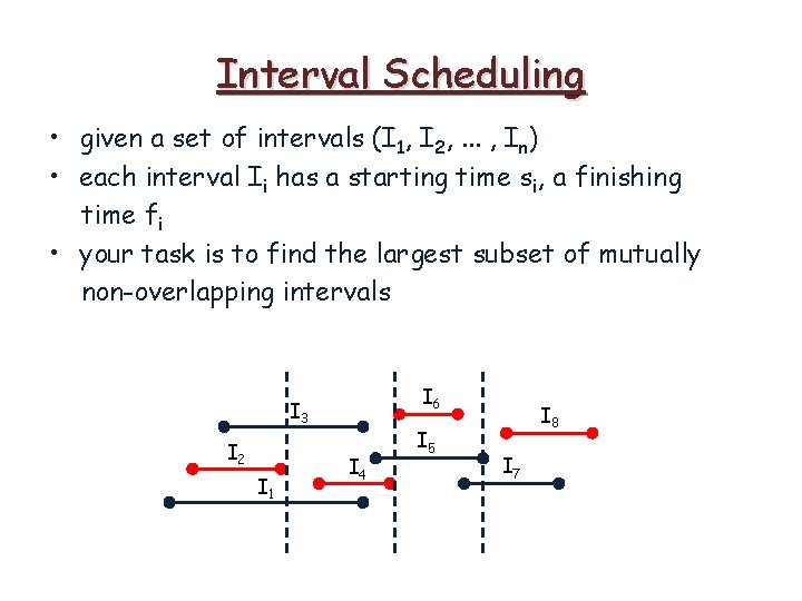
Interval Scheduling • given a set of intervals (I 1, I 2, . . . , In) • each interval Ii has a starting time si, a finishing time fi • your task is to find the largest subset of mutually non-overlapping intervals I 6 I 3 I 2 I 1 I 4 I 5 I 8 I 7

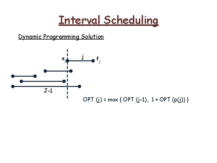
Interval Scheduling Dynamic Programming Solution sj j fj J-1 OPT (j) = max { OPT (j-1), 1 + OPT (p(j)) }

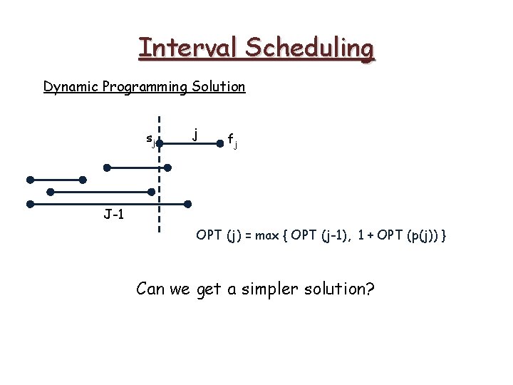
Interval Scheduling Dynamic Programming Solution sj j fj J-1 OPT (j) = max { OPT (j-1), 1 + OPT (p(j)) } Can we get a simpler solution?

Interval Scheduling • solve the problem in myopic fashion (don’t pay attention the global situaton - don’t consider all possible solutions) • make desicion at each step based on improving local state (use greedy approach – pick the one available to you at the moment based on some fixed and simple priority rules)

Interval Scheduling • What is the best option? set the priority rules!

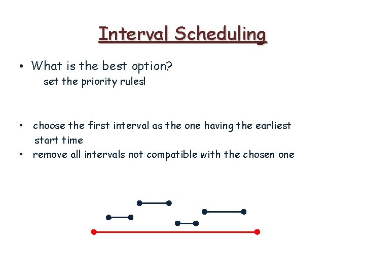
Interval Scheduling • What is the best option? set the priority rules! • choose the first interval as the one having the earliest start time • remove all intervals not compatible with the chosen one

Interval Scheduling • What is the best option? set the priority rules! • choose the first interval as the one having the earliest start time • remove all intervals not compatible with the chosen one

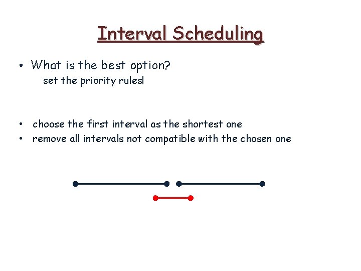
Interval Scheduling • What is the best option? set the priority rules! • choose the first interval as the shortest one • remove all intervals not compatible with the chosen one

Interval Scheduling • What is the best option? set the priority rules! • choose the first interval as the shortest one • remove all intervals not compatible with the chosen one

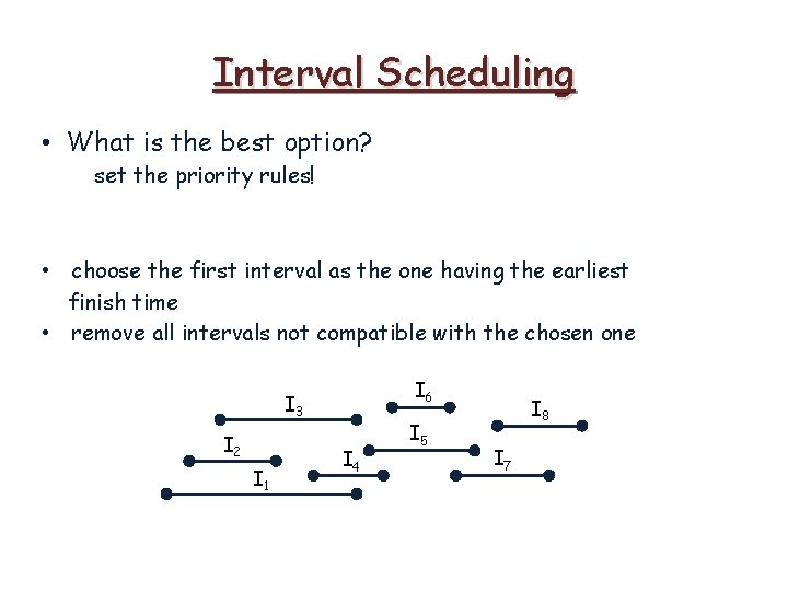
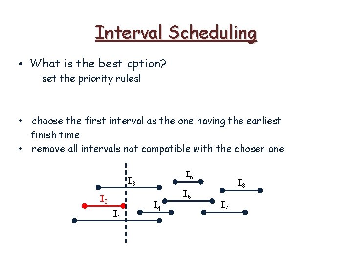
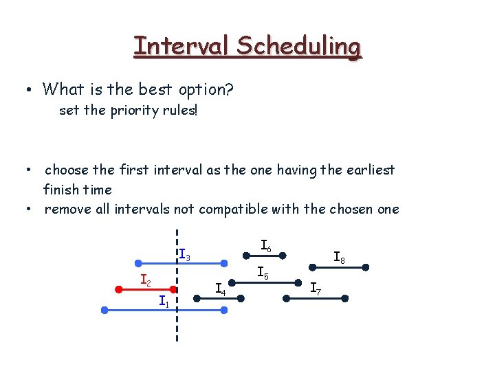
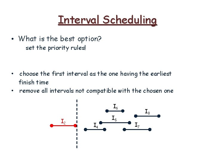
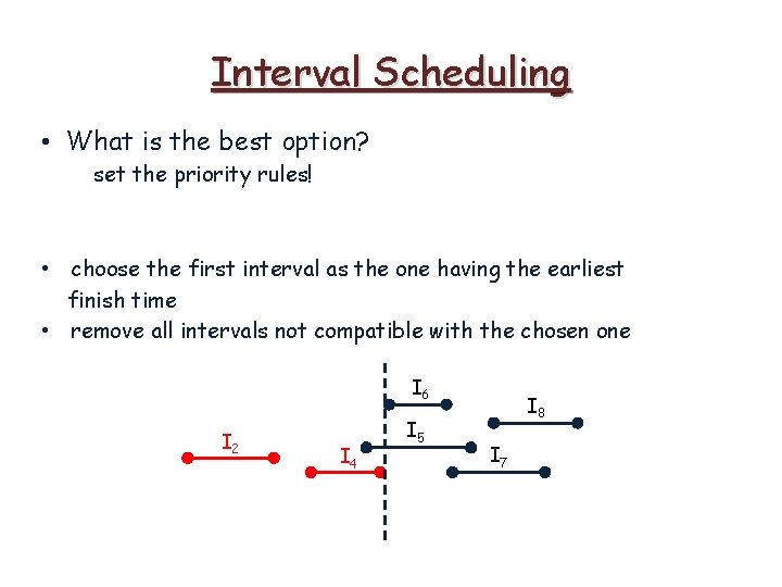
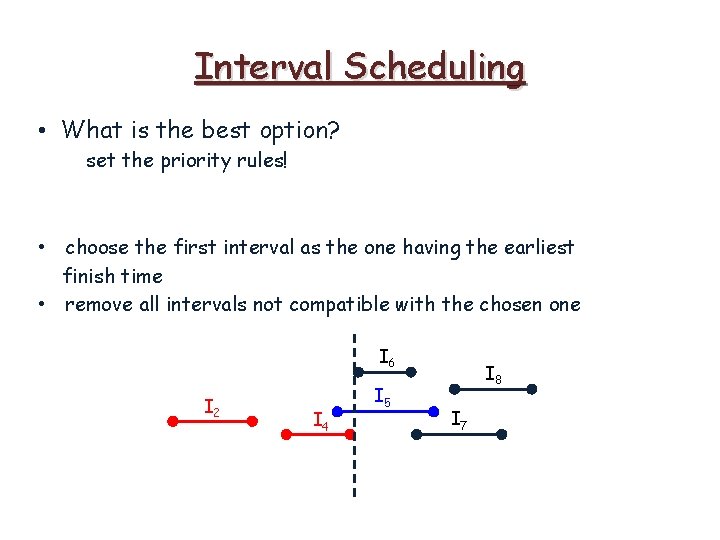
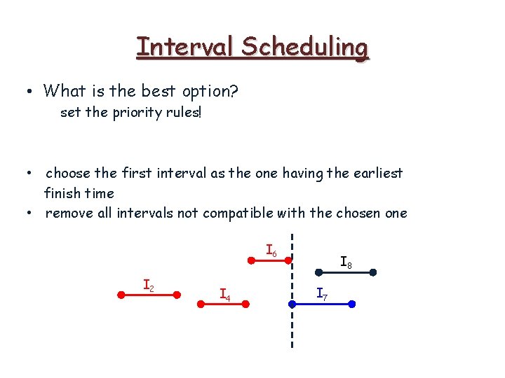
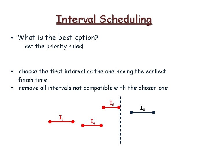
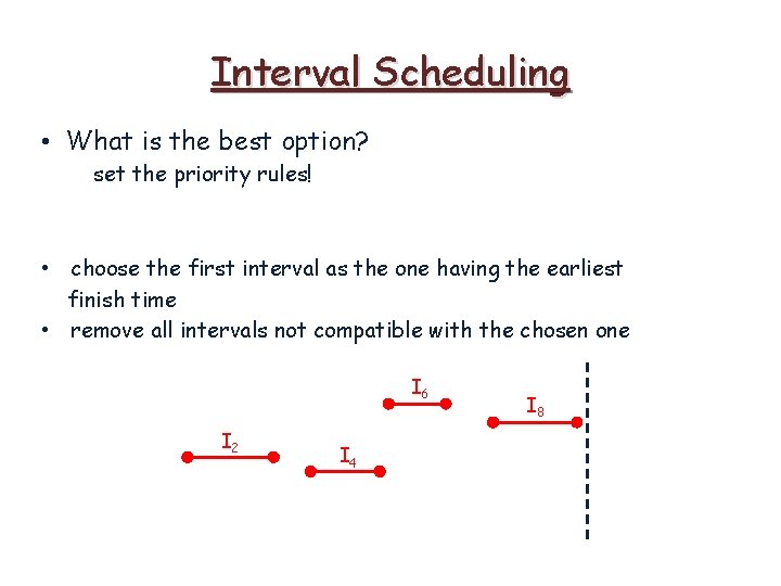
Interval Scheduling • What is the best option? set the priority rules! • choose the first interval as the one having the earliest finish time • remove all intervals not compatible with the chosen one

Interval Scheduling • What is the best option? set the priority rules! • choose the first interval as the one having the earliest finish time • remove all intervals not compatible with the chosen one I 6 I 3 I 2 I 1 I 4 I 5 I 8 I 7

Interval Scheduling • What is the best option? set the priority rules! • choose the first interval as the one having the earliest finish time • remove all intervals not compatible with the chosen one I 6 I 3 I 2 I 1 I 4 I 5 I 8 I 7

Interval Scheduling • What is the best option? set the priority rules! • choose the first interval as the one having the earliest finish time • remove all intervals not compatible with the chosen one I 6 I 3 I 2 I 1 I 4 I 5 I 8 I 7

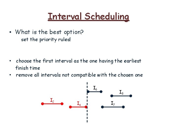
Interval Scheduling • What is the best option? set the priority rules! • choose the first interval as the one having the earliest finish time • remove all intervals not compatible with the chosen one I 6 I 2 I 4 I 5 I 8 I 7

Interval Scheduling • What is the best option? set the priority rules! • choose the first interval as the one having the earliest finish time • remove all intervals not compatible with the chosen one I 6 I 2 I 4 I 5 I 8 I 7

Interval Scheduling • What is the best option? set the priority rules! • choose the first interval as the one having the earliest finish time • remove all intervals not compatible with the chosen one I 6 I 2 I 4 I 5 I 8 I 7

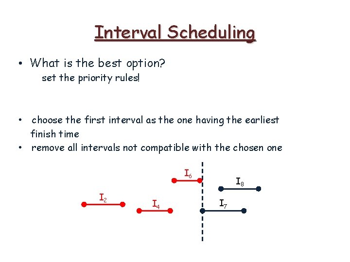
Interval Scheduling • What is the best option? set the priority rules! • choose the first interval as the one having the earliest finish time • remove all intervals not compatible with the chosen one I 6 I 2 I 4 I 8 I 7

Interval Scheduling • What is the best option? set the priority rules! • choose the first interval as the one having the earliest finish time • remove all intervals not compatible with the chosen one I 6 I 2 I 4 I 8 I 7

Interval Scheduling • What is the best option? set the priority rules! • choose the first interval as the one having the earliest finish time • remove all intervals not compatible with the chosen one I 6 I 2 I 4 I 8 I 7

Interval Scheduling • What is the best option? set the priority rules! • choose the first interval as the one having the earliest finish time • remove all intervals not compatible with the chosen one I 6 I 2 I 4 I 8

Interval Scheduling • What is the best option? set the priority rules! • choose the first interval as the one having the earliest finish time • remove all intervals not compatible with the chosen one I 6 I 2 I 4 I 8

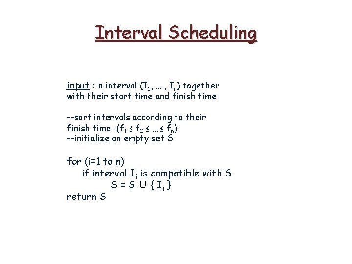
Interval Scheduling input : n interval (I 1, … , In) together with their start time and finish time --sort intervals according to their finish time (f 1 ≤ f 2 ≤ … ≤ fn) --initialize an empty set S for (i=1 to n) if interval Ii is compatible with S S = S ∪ { Ii } return S

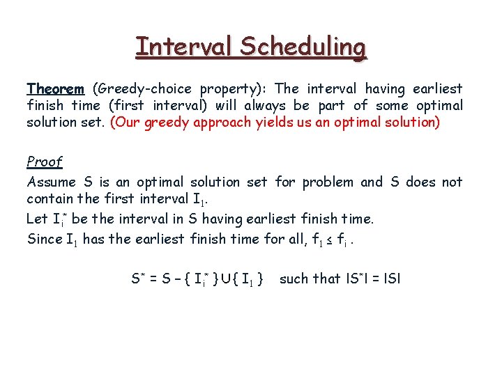
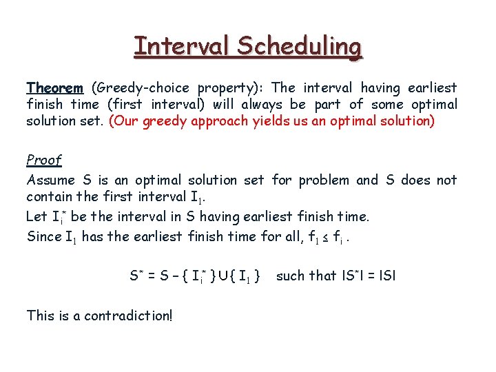
Interval Scheduling Theorem (Greedy-choice property): The interval having earliest finish time (first interval) will always be part of some optimal solution set. (Our greedy approach yields us an optimal solution) Proof

Interval Scheduling Theorem (Greedy-choice property): The interval having earliest finish time (first interval) will always be part of some optimal solution set. (Our greedy approach yields us an optimal solution) Proof Assume S is an optimal solution set for problem and S does not contain the first interval I 1.

Interval Scheduling Theorem (Greedy-choice property): The interval having earliest finish time (first interval) will always be part of some optimal solution set. (Our greedy approach yields us an optimal solution) Proof Assume S is an optimal solution set for problem and S does not contain the first interval I 1. Let Ii* be the interval in S having earliest finish time.

Interval Scheduling Theorem (Greedy-choice property): The interval having earliest finish time (first interval) will always be part of some optimal solution set. (Our greedy approach yields us an optimal solution) Proof Assume S is an optimal solution set for problem and S does not contain the first interval I 1. Let Ii* be the interval in S having earliest finish time. Since I 1 has the earliest finish time for all, f 1 ≤ fi.

Interval Scheduling Theorem (Greedy-choice property): The interval having earliest finish time (first interval) will always be part of some optimal solution set. (Our greedy approach yields us an optimal solution) Proof Assume S is an optimal solution set for problem and S does not contain the first interval I 1. Let Ii* be the interval in S having earliest finish time. Since I 1 has the earliest finish time for all, f 1 ≤ fi. S* = S – { Ii* }∪{ I 1 } such that ΙS*Ι = ΙSΙ

Interval Scheduling Theorem (Greedy-choice property): The interval having earliest finish time (first interval) will always be part of some optimal solution set. (Our greedy approach yields us an optimal solution) Proof Assume S is an optimal solution set for problem and S does not contain the first interval I 1. Let Ii* be the interval in S having earliest finish time. Since I 1 has the earliest finish time for all, f 1 ≤ fi. S* = S – { Ii* }∪{ I 1 } This is a contradiction! such that ΙS*Ι = ΙSΙ

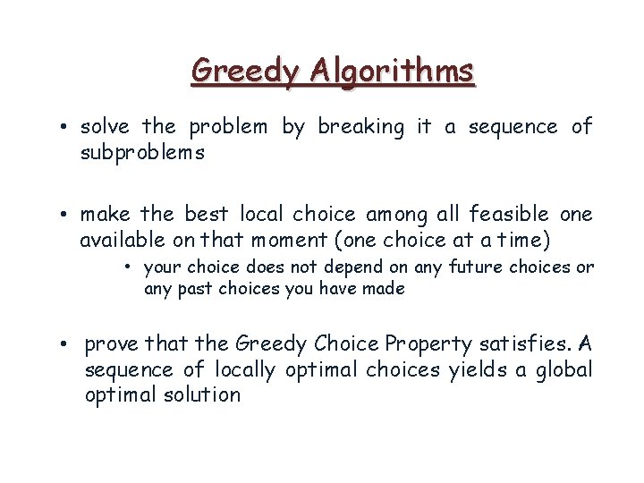
Greedy Algorithms • solve the problem by breaking it a sequence of subproblems • make the best local choice among all feasible one available on that moment (one choice at a time) • your choice does not depend on any future choices or any past choices you have made • prove that the Greedy Choice Property satisfies. A sequence of locally optimal choices yields a global optimal solution

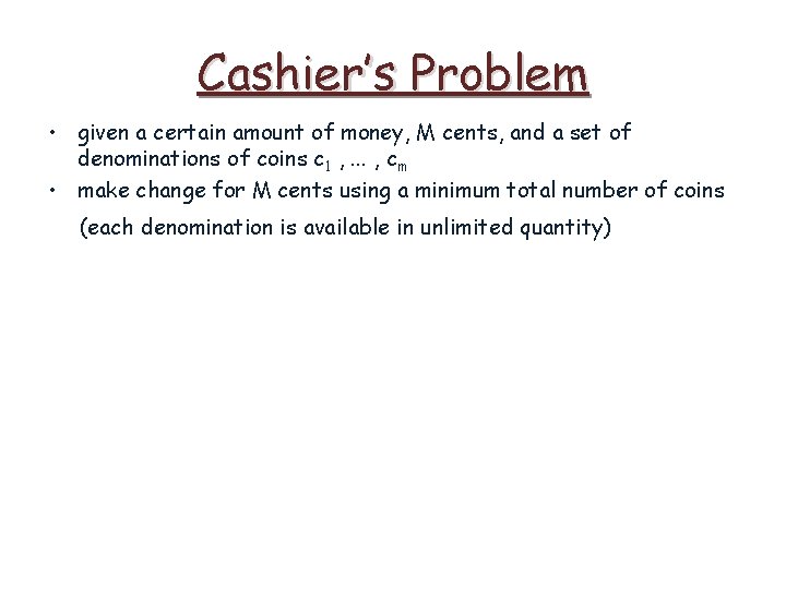
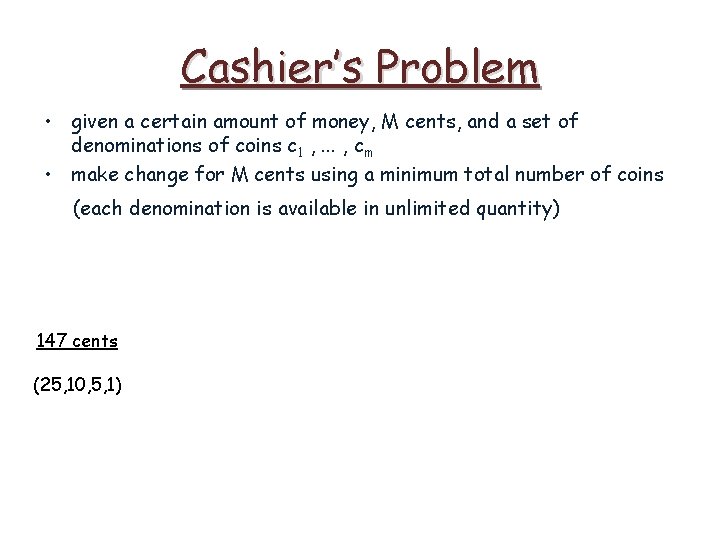
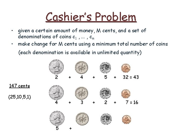
Cashier’s Problem • given a certain amount of money, M cents, and a set of denominations of coins c 1 , . . . , cm • make change for M cents using a minimum total number of coins (each denomination is available in unlimited quantity)

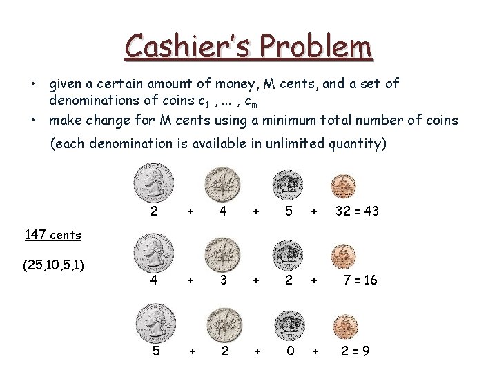
Cashier’s Problem • given a certain amount of money, M cents, and a set of denominations of coins c 1 , . . . , cm • make change for M cents using a minimum total number of coins (each denomination is available in unlimited quantity) 147 cents (25, 10, 5, 1)

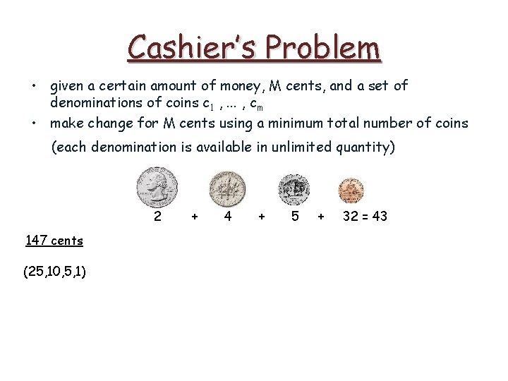
Cashier’s Problem • given a certain amount of money, M cents, and a set of denominations of coins c 1 , . . . , cm • make change for M cents using a minimum total number of coins (each denomination is available in unlimited quantity) 2 147 cents (25, 10, 5, 1) + 4 + 5 + 32 = 43

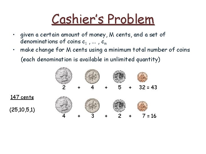
Cashier’s Problem • given a certain amount of money, M cents, and a set of denominations of coins c 1 , . . . , cm • make change for M cents using a minimum total number of coins (each denomination is available in unlimited quantity) 2 + 4 + 5 + 32 = 43 4 + 3 + 2 + 7 = 16 147 cents (25, 10, 5, 1)

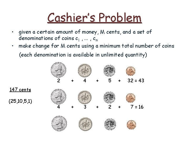
Cashier’s Problem • given a certain amount of money, M cents, and a set of denominations of coins c 1 , . . . , cm • make change for M cents using a minimum total number of coins (each denomination is available in unlimited quantity) 2 + 4 + 5 + 32 = 43 4 + 3 + 2 + 7 = 16 147 cents (25, 10, 5, 1)

Cashier’s Problem • given a certain amount of money, M cents, and a set of denominations of coins c 1 , . . . , cm • make change for M cents using a minimum total number of coins (each denomination is available in unlimited quantity) 2 + 4 + 5 + 32 = 43 4 + 3 + 2 + 7 = 16 5 + 147 cents (25, 10, 5, 1)

Cashier’s Problem • given a certain amount of money, M cents, and a set of denominations of coins c 1 , . . . , cm • make change for M cents using a minimum total number of coins (each denomination is available in unlimited quantity) 2 + 4 + 5 + 32 = 43 4 + 3 + 2 + 7 = 16 5 + 2 + 147 cents (25, 10, 5, 1)

Cashier’s Problem • given a certain amount of money, M cents, and a set of denominations of coins c 1 , . . . , cm • make change for M cents using a minimum total number of coins (each denomination is available in unlimited quantity) 2 + 4 + 5 + 32 = 43 4 + 3 + 2 + 7 = 16 5 + 2 + 0 + 147 cents (25, 10, 5, 1)

Cashier’s Problem • given a certain amount of money, M cents, and a set of denominations of coins c 1 , . . . , cm • make change for M cents using a minimum total number of coins (each denomination is available in unlimited quantity) 2 + 4 + 5 + 32 = 43 4 + 3 + 2 + 7 = 16 5 + 2 + 0 + 2=9 147 cents (25, 10, 5, 1)

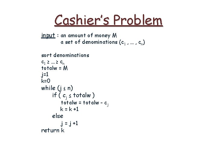
Cashier’s Problem input : an amount of money M a set of denominations (c 1 , … , cn) sort denominations c 1 ≥ … ≥ c n totalw = M j=1 k=0 while (j ≤ n) if ( cj ≤ totalw ) totalw = totalw - cj k = k +1 else j = j +1 return k

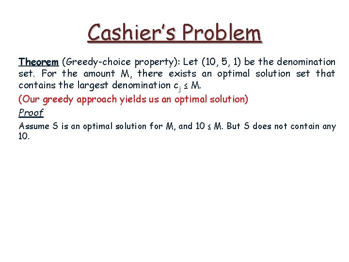
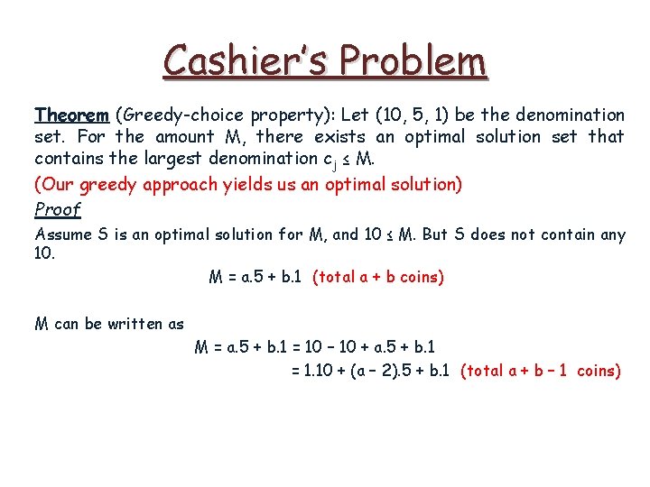
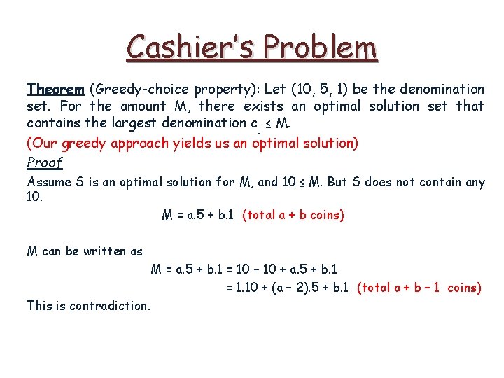
Cashier’s Problem Theorem (Greedy-choice property): Let (10, 5, 1) be the denomination set. For the amount M, there exists an optimal solution set that contains the largest denomination cj ≤ M. (Our greedy approach yields us an optimal solution) Proof

Cashier’s Problem Theorem (Greedy-choice property): Let (10, 5, 1) be the denomination set. For the amount M, there exists an optimal solution set that contains the largest denomination cj ≤ M. (Our greedy approach yields us an optimal solution) Proof Assume S is an optimal solution for M, and 10 ≤ M. But S does not contain any 10.

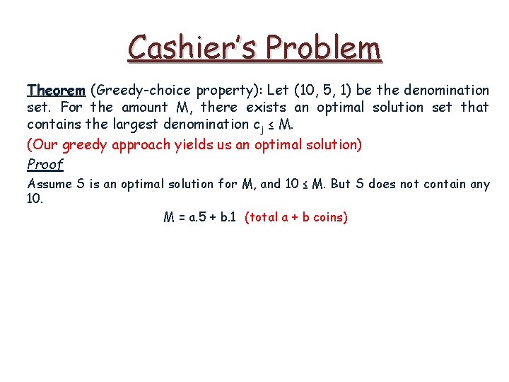
Cashier’s Problem Theorem (Greedy-choice property): Let (10, 5, 1) be the denomination set. For the amount M, there exists an optimal solution set that contains the largest denomination cj ≤ M. (Our greedy approach yields us an optimal solution) Proof Assume S is an optimal solution for M, and 10 ≤ M. But S does not contain any 10. M = a. 5 + b. 1 (total a + b coins)

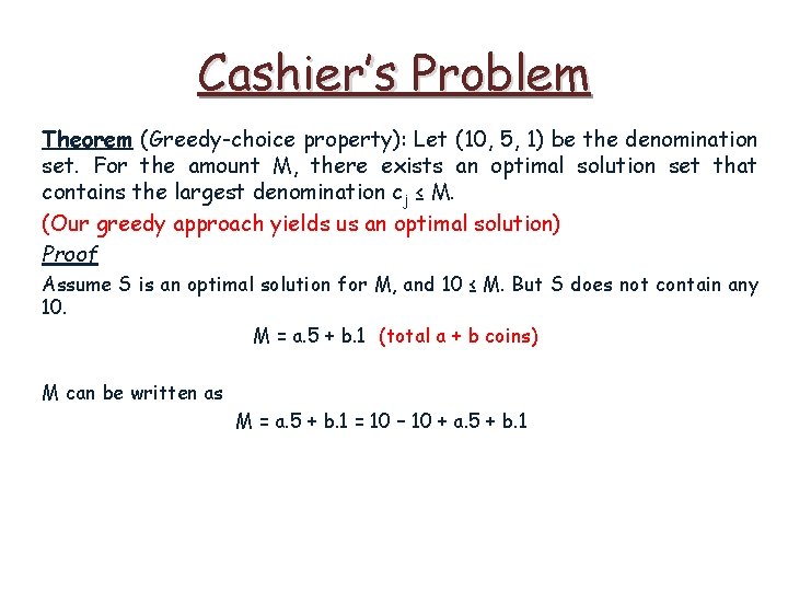
Cashier’s Problem Theorem (Greedy-choice property): Let (10, 5, 1) be the denomination set. For the amount M, there exists an optimal solution set that contains the largest denomination cj ≤ M. (Our greedy approach yields us an optimal solution) Proof Assume S is an optimal solution for M, and 10 ≤ M. But S does not contain any 10. M = a. 5 + b. 1 (total a + b coins) M can be written as M = a. 5 + b. 1 = 10 – 10 + a. 5 + b. 1

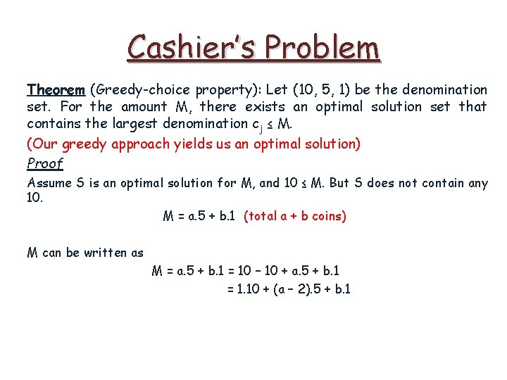
Cashier’s Problem Theorem (Greedy-choice property): Let (10, 5, 1) be the denomination set. For the amount M, there exists an optimal solution set that contains the largest denomination cj ≤ M. (Our greedy approach yields us an optimal solution) Proof Assume S is an optimal solution for M, and 10 ≤ M. But S does not contain any 10. M = a. 5 + b. 1 (total a + b coins) M can be written as M = a. 5 + b. 1 = 10 – 10 + a. 5 + b. 1 = 1. 10 + (a – 2). 5 + b. 1

Cashier’s Problem Theorem (Greedy-choice property): Let (10, 5, 1) be the denomination set. For the amount M, there exists an optimal solution set that contains the largest denomination cj ≤ M. (Our greedy approach yields us an optimal solution) Proof Assume S is an optimal solution for M, and 10 ≤ M. But S does not contain any 10. M = a. 5 + b. 1 (total a + b coins) M can be written as M = a. 5 + b. 1 = 10 – 10 + a. 5 + b. 1 = 1. 10 + (a – 2). 5 + b. 1 (total a + b – 1 coins)

Cashier’s Problem Theorem (Greedy-choice property): Let (10, 5, 1) be the denomination set. For the amount M, there exists an optimal solution set that contains the largest denomination cj ≤ M. (Our greedy approach yields us an optimal solution) Proof Assume S is an optimal solution for M, and 10 ≤ M. But S does not contain any 10. M = a. 5 + b. 1 (total a + b coins) M can be written as M = a. 5 + b. 1 = 10 – 10 + a. 5 + b. 1 = 1. 10 + (a – 2). 5 + b. 1 (total a + b – 1 coins) This is contradiction.

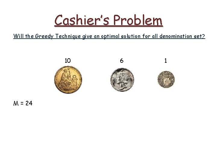
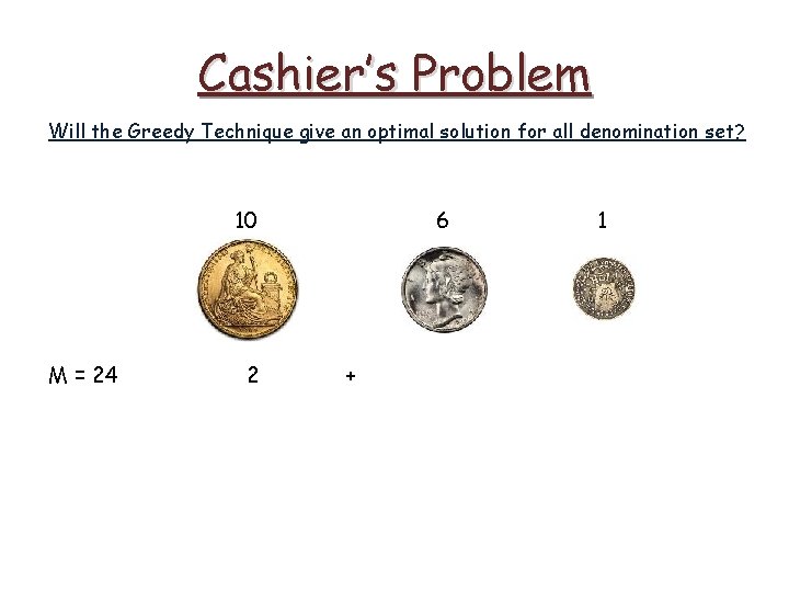
Cashier’s Problem Will the Greedy Technique give an optimal solution for all denomination set?

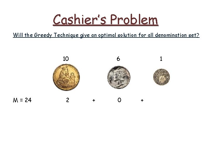
Cashier’s Problem Will the Greedy Technique give an optimal solution for all denomination set? 10 M = 24 6 1

Cashier’s Problem Will the Greedy Technique give an optimal solution for all denomination set? 10 M = 24 2 6 + 1

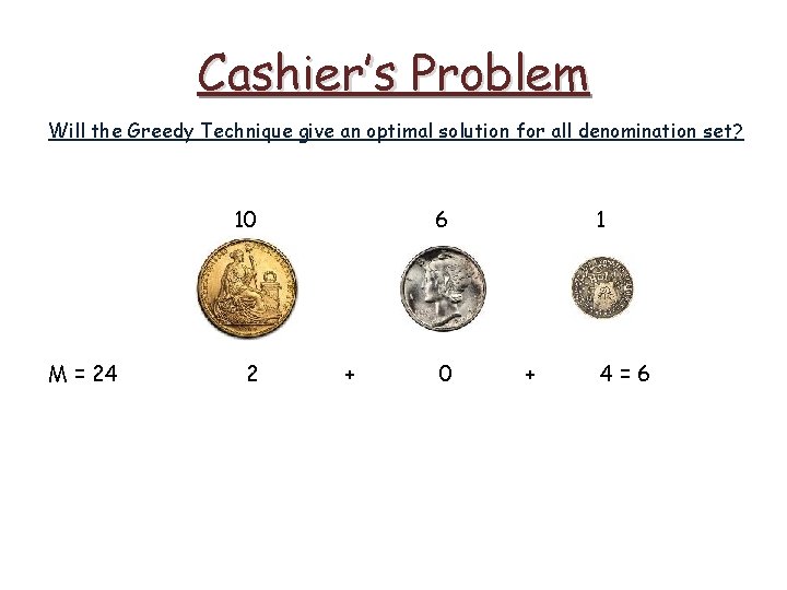
Cashier’s Problem Will the Greedy Technique give an optimal solution for all denomination set? 10 M = 24 2 6 + 0 1 +

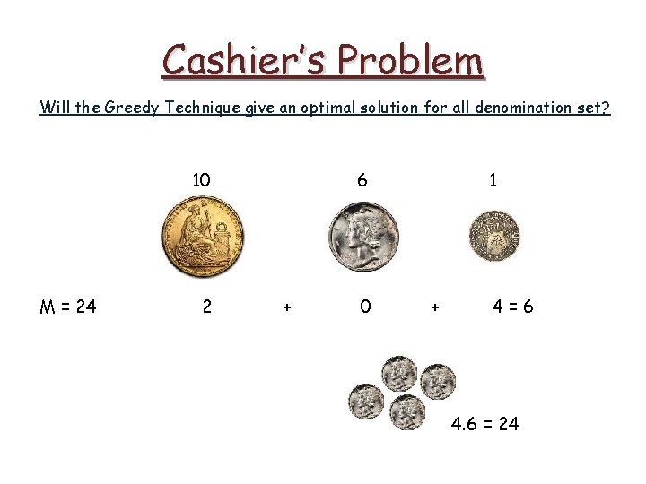
Cashier’s Problem Will the Greedy Technique give an optimal solution for all denomination set? 10 M = 24 2 6 + 0 1 + 4=6

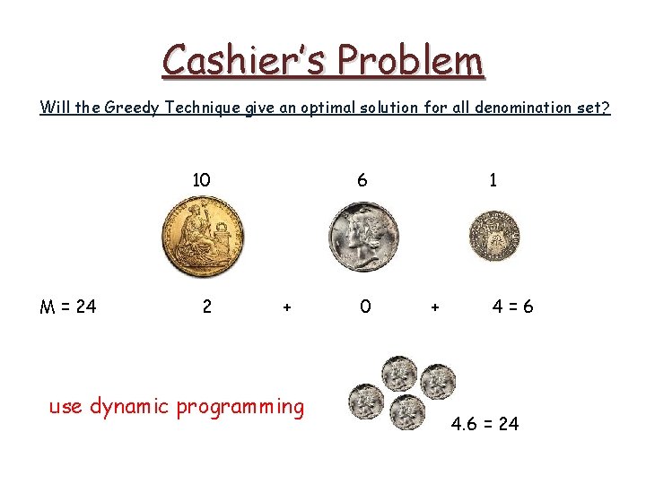
Cashier’s Problem Will the Greedy Technique give an optimal solution for all denomination set? 10 M = 24 2 6 + 0 1 + 4=6 4. 6 = 24

Cashier’s Problem Will the Greedy Technique give an optimal solution for all denomination set? 10 M = 24 2 6 + use dynamic programming 0 1 + 4=6 4. 6 = 24

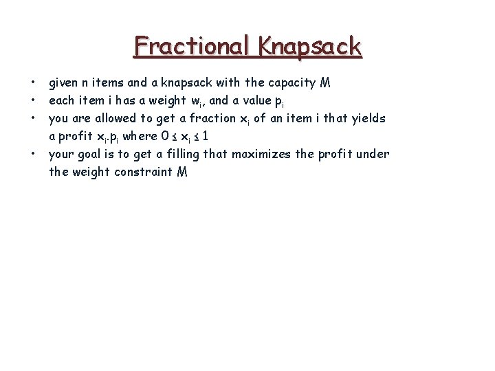
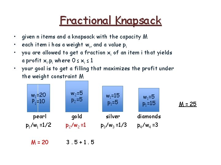
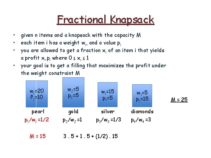
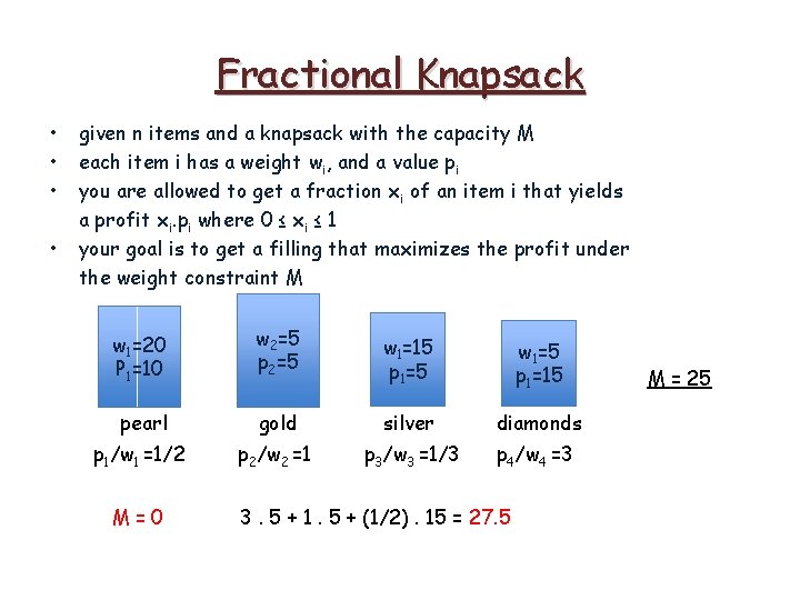
Fractional Knapsack • • given n items and a knapsack with the capacity M each item i has a weight wi, and a value pi you are allowed to get a fraction xi of an item i that yields a profit xi. pi where 0 ≤ xi ≤ 1 your goal is to get a filling that maximizes the profit under the weight constraint M

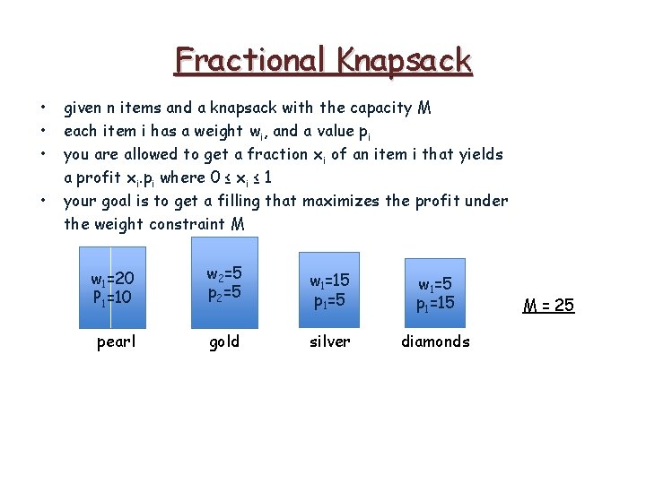
Fractional Knapsack • • given n items and a knapsack with the capacity M each item i has a weight wi, and a value pi you are allowed to get a fraction xi of an item i that yields a profit xi. pi where 0 ≤ xi ≤ 1 your goal is to get a filling that maximizes the profit under the weight constraint M w 1=20 P 1=10 w 2=5 p 2=5 w 1=15 p 1=5 w 1=5 p 1=15 pearl gold silver diamonds M = 25

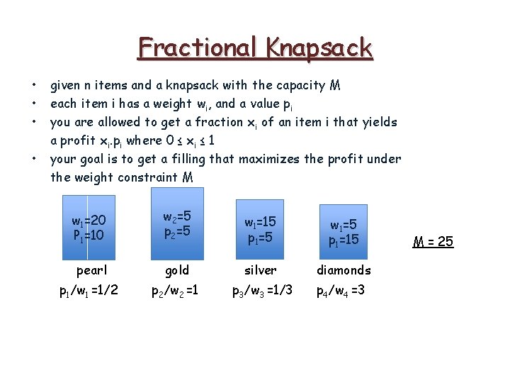
Fractional Knapsack • • given n items and a knapsack with the capacity M each item i has a weight wi, and a value pi you are allowed to get a fraction xi of an item i that yields a profit xi. pi where 0 ≤ xi ≤ 1 your goal is to get a filling that maximizes the profit under the weight constraint M w 1=20 P 1=10 w 2=5 p 2=5 w 1=15 p 1=5 w 1=5 p 1=15 pearl gold silver diamonds p 1/w 1 =1/2 p 2/w 2 =1 p 3/w 3 =1/3 p 4/w 4 =3 M = 25

Fractional Knapsack • • given n items and a knapsack with the capacity M each item i has a weight wi, and a value pi you are allowed to get a fraction xi of an item i that yields a profit xi. pi where 0 ≤ xi ≤ 1 your goal is to get a filling that maximizes the profit under the weight constraint M w 1=20 P 1=10 w 2=5 p 2=5 w 1=15 p 1=5 w 1=5 p 1=15 pearl gold silver diamonds p 1/w 1 =1/2 p 2/w 2 =1 p 3/w 3 =1/3 p 4/w 4 =3 M = 25

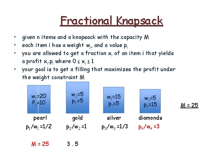
Fractional Knapsack • • given n items and a knapsack with the capacity M each item i has a weight wi, and a value pi you are allowed to get a fraction xi of an item i that yields a profit xi. pi where 0 ≤ xi ≤ 1 your goal is to get a filling that maximizes the profit under the weight constraint M w 1=20 P 1=10 w 2=5 p 2=5 w 1=15 p 1=5 w 1=5 p 1=15 pearl gold silver diamonds p 1/w 1 =1/2 p 2/w 2 =1 p 3/w 3 =1/3 p 4/w 4 =3 M = 25 3. 5 M = 25

Fractional Knapsack • • given n items and a knapsack with the capacity M each item i has a weight wi, and a value pi you are allowed to get a fraction xi of an item i that yields a profit xi. pi where 0 ≤ xi ≤ 1 your goal is to get a filling that maximizes the profit under the weight constraint M w 1=20 P 1=10 w 2=5 p 2=5 w 1=15 p 1=5 w 1=5 p 1=15 pearl gold silver diamonds p 1/w 1 =1/2 p 2/w 2 =1 p 3/w 3 =1/3 p 4/w 4 =3 M = 20 3. 5+1. 5 M = 25

Fractional Knapsack • • given n items and a knapsack with the capacity M each item i has a weight wi, and a value pi you are allowed to get a fraction xi of an item i that yields a profit xi. pi where 0 ≤ xi ≤ 1 your goal is to get a filling that maximizes the profit under the weight constraint M w 1=20 P 1=10 w 2=5 p 2=5 w 1=15 p 1=5 w 1=5 p 1=15 pearl gold silver diamonds p 1/w 1 =1/2 p 2/w 2 =1 p 3/w 3 =1/3 p 4/w 4 =3 M = 15 3. 5 + 1. 5 + (1/2). 15 M = 25

Fractional Knapsack • • given n items and a knapsack with the capacity M each item i has a weight wi, and a value pi you are allowed to get a fraction xi of an item i that yields a profit xi. pi where 0 ≤ xi ≤ 1 your goal is to get a filling that maximizes the profit under the weight constraint M w 1=20 P 1=10 w 2=5 p 2=5 w 1=15 p 1=5 w 1=5 p 1=15 pearl gold silver diamonds p 1/w 1 =1/2 p 2/w 2 =1 p 3/w 3 =1/3 p 4/w 4 =3 M=0 3. 5 + 1. 5 + (1/2). 15 = 27. 5 M = 25

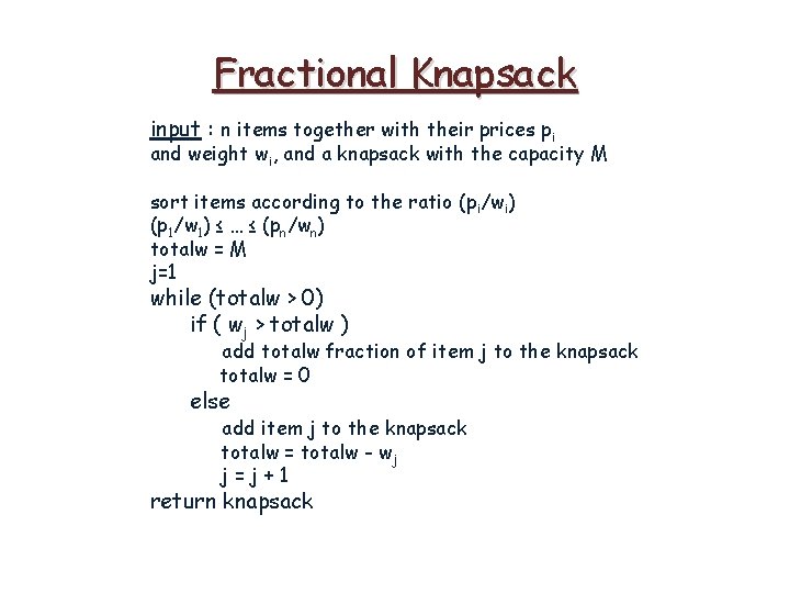
Fractional Knapsack input : n items together with their prices pi and weight wi, and a knapsack with the capacity M sort items according to the ratio (pi/wi) (p 1/w 1) ≤ … ≤ (pn/wn) totalw = M j=1 while (totalw > 0) if ( wj > totalw ) add totalw fraction of item j to the knapsack totalw = 0 else add item j to the knapsack totalw = totalw - wj j=j+1 return knapsack

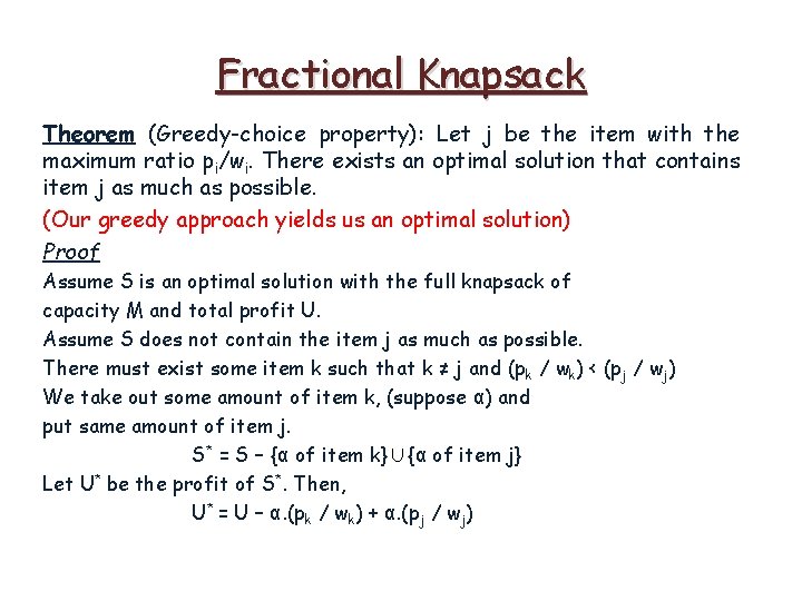
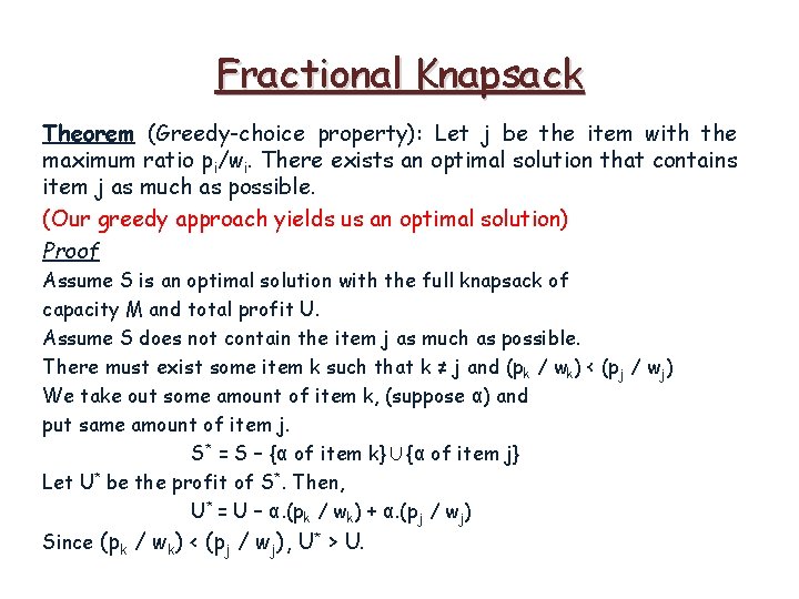
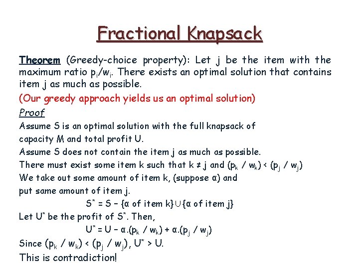
Fractional Knapsack Theorem (Greedy-choice property): Let j be the item with the maximum ratio pi/wi. There exists an optimal solution that contains item j as much as possible. (Our greedy approach yields us an optimal solution) Proof

Fractional Knapsack Theorem (Greedy-choice property): Let j be the item with the maximum ratio pi/wi. There exists an optimal solution that contains item j as much as possible. (Our greedy approach yields us an optimal solution) Proof Assume S is an optimal solution with the full knapsack of capacity M and total profit U.

Fractional Knapsack Theorem (Greedy-choice property): Let j be the item with the maximum ratio pi/wi. There exists an optimal solution that contains item j as much as possible. (Our greedy approach yields us an optimal solution) Proof Assume S is an optimal solution with the full knapsack of capacity M and total profit U. Assume S does not contain the item j as much as possible. There must exist some item k such that k ≠ j and (p k / wk) < (pj / wj)

Fractional Knapsack Theorem (Greedy-choice property): Let j be the item with the maximum ratio pi/wi. There exists an optimal solution that contains item j as much as possible. (Our greedy approach yields us an optimal solution) Proof Assume S is an optimal solution with the full knapsack of capacity M and total profit U. Assume S does not contain the item j as much as possible. There must exist some item k such that k ≠ j and (p k / wk) < (pj / wj) We take out some amount of item k, (suppose α) and put same amount of item j. S* = S – {α of item k}∪{α of item j}

Fractional Knapsack Theorem (Greedy-choice property): Let j be the item with the maximum ratio pi/wi. There exists an optimal solution that contains item j as much as possible. (Our greedy approach yields us an optimal solution) Proof Assume S is an optimal solution with the full knapsack of capacity M and total profit U. Assume S does not contain the item j as much as possible. There must exist some item k such that k ≠ j and (p k / wk) < (pj / wj) We take out some amount of item k, (suppose α) and put same amount of item j. S* = S – {α of item k}∪{α of item j} Let U* be the profit of S*. Then, U* = U – α. (pk / wk) + α. (pj / wj)

Fractional Knapsack Theorem (Greedy-choice property): Let j be the item with the maximum ratio pi/wi. There exists an optimal solution that contains item j as much as possible. (Our greedy approach yields us an optimal solution) Proof Assume S is an optimal solution with the full knapsack of capacity M and total profit U. Assume S does not contain the item j as much as possible. There must exist some item k such that k ≠ j and (p k / wk) < (pj / wj) We take out some amount of item k, (suppose α) and put same amount of item j. S* = S – {α of item k}∪{α of item j} Let U* be the profit of S*. Then, U* = U – α. (pk / wk) + α. (pj / wj) Since (pk / wk) < (pj / wj), U* > U.

Fractional Knapsack Theorem (Greedy-choice property): Let j be the item with the maximum ratio pi/wi. There exists an optimal solution that contains item j as much as possible. (Our greedy approach yields us an optimal solution) Proof Assume S is an optimal solution with the full knapsack of capacity M and total profit U. Assume S does not contain the item j as much as possible. There must exist some item k such that k ≠ j and (p k / wk) < (pj / wj) We take out some amount of item k, (suppose α) and put same amount of item j. S* = S – {α of item k}∪{α of item j} Let U* be the profit of S*. Then, U* = U – α. (pk / wk) + α. (pj / wj) Since (pk / wk) < (pj / wj), U* > U. This is contradiction!

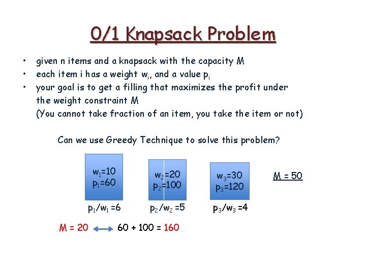
0/1 Knapsack Problem • • • given n items and a knapsack with the capacity M each item i has a weight wi, and a value pi your goal is to get a filling that maximizes the profit under the weight constraint M (You cannot take fraction of an item, you take the item or not)

0/1 Knapsack Problem • • • given n items and a knapsack with the capacity M each item i has a weight wi, and a value pi your goal is to get a filling that maximizes the profit under the weight constraint M (You cannot take fraction of an item, you take the item or not) Can we use Greedy Technique to solve this problem?

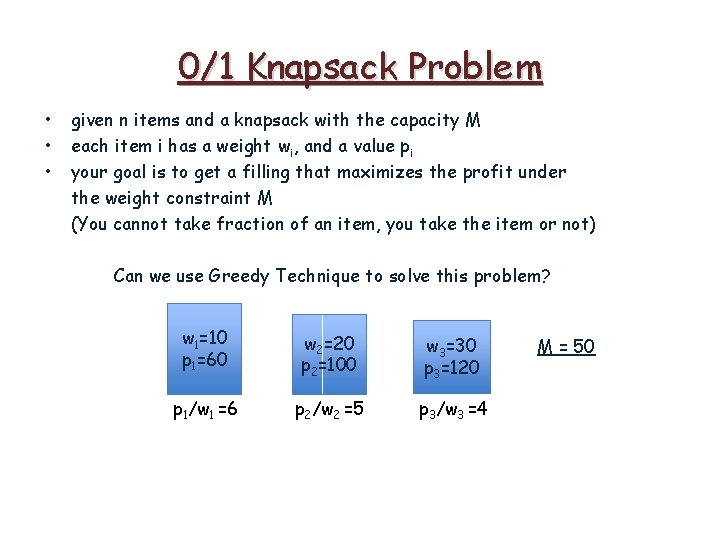
0/1 Knapsack Problem • • • given n items and a knapsack with the capacity M each item i has a weight wi, and a value pi your goal is to get a filling that maximizes the profit under the weight constraint M (You cannot take fraction of an item, you take the item or not) Can we use Greedy Technique to solve this problem? w 1=10 p 1=60 w 2=20 p 2=100 w 3=30 p 3=120 p 1/w 1 =6 p 2/w 2 =5 p 3/w 3 =4 M = 50

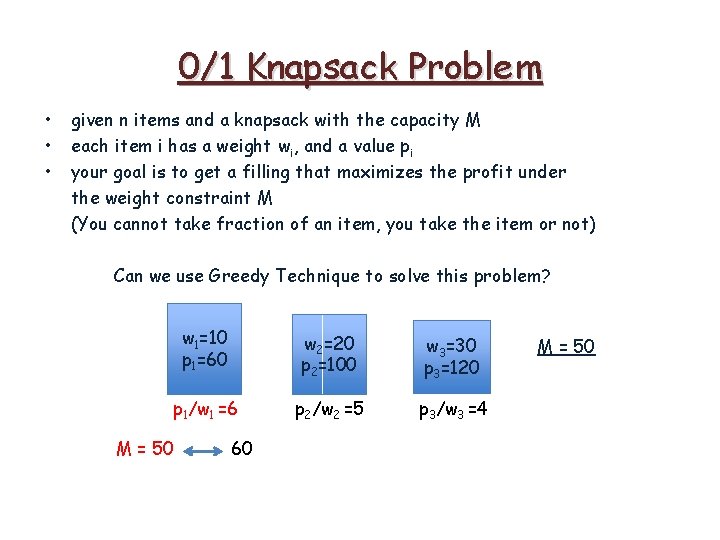
0/1 Knapsack Problem • • • given n items and a knapsack with the capacity M each item i has a weight wi, and a value pi your goal is to get a filling that maximizes the profit under the weight constraint M (You cannot take fraction of an item, you take the item or not) Can we use Greedy Technique to solve this problem? w 1=10 p 1=60 w 2=20 p 2=100 w 3=30 p 3=120 p 1/w 1 =6 p 2/w 2 =5 p 3/w 3 =4 M = 50 60 M = 50

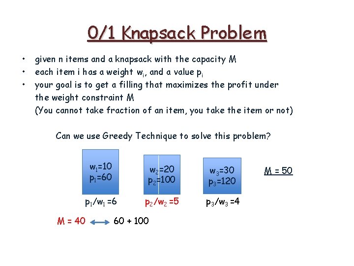
0/1 Knapsack Problem • • • given n items and a knapsack with the capacity M each item i has a weight wi, and a value pi your goal is to get a filling that maximizes the profit under the weight constraint M (You cannot take fraction of an item, you take the item or not) Can we use Greedy Technique to solve this problem? w 1=10 p 1=60 w 2=20 p 2=100 w 3=30 p 3=120 p 1/w 1 =6 p 2/w 2 =5 p 3/w 3 =4 M = 40 60 + 100 M = 50

0/1 Knapsack Problem • • • given n items and a knapsack with the capacity M each item i has a weight wi, and a value pi your goal is to get a filling that maximizes the profit under the weight constraint M (You cannot take fraction of an item, you take the item or not) Can we use Greedy Technique to solve this problem? w 1=10 p 1=60 w 2=20 p 2=100 w 3=30 p 3=120 p 1/w 1 =6 p 2/w 2 =5 p 3/w 3 =4 M = 20 60 + 100 = 160 M = 50

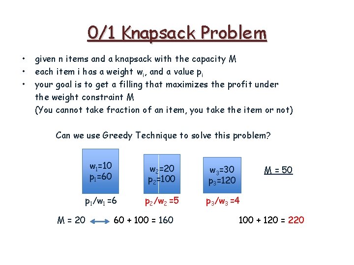
0/1 Knapsack Problem • • • given n items and a knapsack with the capacity M each item i has a weight wi, and a value pi your goal is to get a filling that maximizes the profit under the weight constraint M (You cannot take fraction of an item, you take the item or not) Can we use Greedy Technique to solve this problem? w 1=10 p 1=60 w 2=20 p 2=100 w 3=30 p 3=120 p 1/w 1 =6 p 2/w 2 =5 p 3/w 3 =4 M = 20 60 + 100 = 160 M = 50 100 + 120 = 220

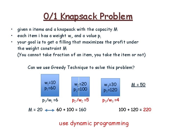
0/1 Knapsack Problem • • • given n items and a knapsack with the capacity M each item i has a weight wi, and a value pi your goal is to get a filling that maximizes the profit under the weight constraint M (You cannot take fraction of an item, you take the item or not) Can we use Greedy Technique to solve this problem? w 1=10 p 1=60 w 2=20 p 2=100 w 3=30 p 3=120 p 1/w 1 =6 p 2/w 2 =5 p 3/w 3 =4 M = 20 60 + 100 = 160 M = 50 100 + 120 = 220 use dynamic programming

Process Scheduling • given a computer and n processes p 1, . . . , pn such that each of them has a completion time ti • find an optimal order of processes that has the minimum average finishing time

Process Scheduling • given a computer and n processes p 1, . . . , pn such that each of them has a completion time ti • find an optimal order of processes that has the minimum average finishing time If we define the finishing time C i of the process i as Ci = Σj=1. . itj , then the average finishing time will be (Σ i=1. . n Ci)/n.

Process Scheduling • given a computer and n processes p 1, . . . , pn such that each of them has a completion time ti • find an optimal order of processes that has the minimum average finishing time If we define the finishing time C i of the process i as Ci = Σj=1. . itj , then the average finishing time will be (Σ i=1. . n Ci)/n. Our goal is to minimize (Σi=1. . n Ci)/n

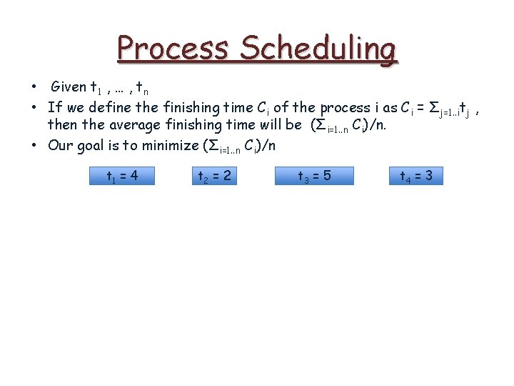
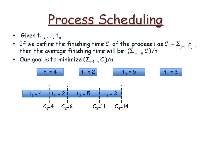
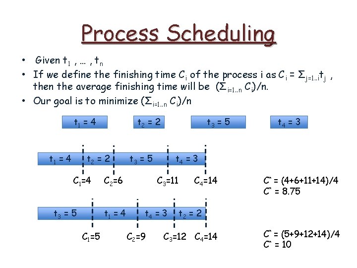
Process Scheduling • Given t 1 , … , tn • If we define the finishing time Ci of the process i as Ci = Σj=1. . itj , then the average finishing time will be (Σi=1. . n Ci)/n. • Our goal is to minimize (Σi=1. . n Ci)/n t 1 = 4 t 2 = 2 t 3 = 5 t 4 = 3

Process Scheduling • Given t 1 , … , tn • If we define the finishing time Ci of the process i as Ci = Σj=1. . itj , then the average finishing time will be (Σi=1. . n Ci)/n. • Our goal is to minimize (Σi=1. . n Ci)/n t 1 = 4 t 2 = 2 t 3 = 5 t 4 = 3

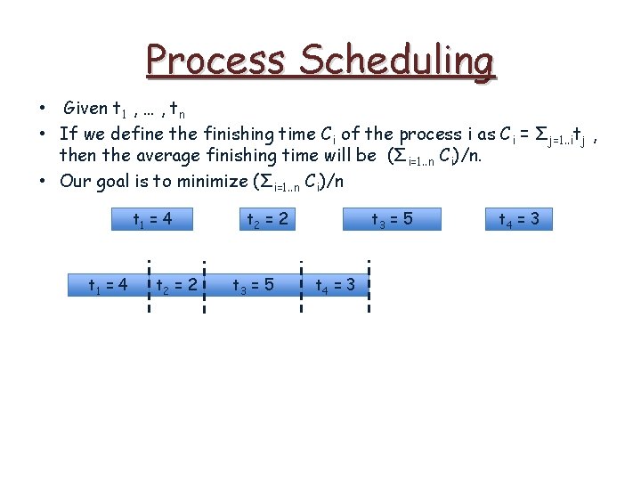
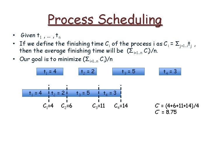
Process Scheduling • Given t 1 , … , tn • If we define the finishing time Ci of the process i as Ci = Σj=1. . itj , then the average finishing time will be (Σi=1. . n Ci)/n. • Our goal is to minimize (Σi=1. . n Ci)/n t 1 = 4 t 2 = 2 C 1=4 C 2=6 t 3 = 5 t 4 = 3 C 3=11 C 4=14 t 4 = 3

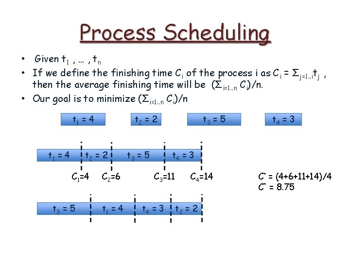
Process Scheduling • Given t 1 , … , tn • If we define the finishing time Ci of the process i as Ci = Σj=1. . itj , then the average finishing time will be (Σi=1. . n Ci)/n. • Our goal is to minimize (Σi=1. . n Ci)/n t 1 = 4 t 2 = 2 C 1=4 C 2=6 t 3 = 5 t 4 = 3 C 3=11 C 4=14 C* = (4+6+11+14)/4 C* = 8. 75

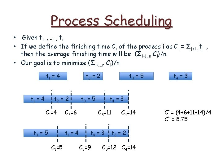
Process Scheduling • Given t 1 , … , tn • If we define the finishing time Ci of the process i as Ci = Σj=1. . itj , then the average finishing time will be (Σi=1. . n Ci)/n. • Our goal is to minimize (Σi=1. . n Ci)/n t 1 = 4 t 2 = 2 C 1=4 t 3 = 5 C 2=6 t 1 = 4 t 3 = 5 t 4 = 3 C 3=11 t 4 = 3 C 4=14 t 2 = 2 C* = (4+6+11+14)/4 C* = 8. 75

Process Scheduling • Given t 1 , … , tn • If we define the finishing time Ci of the process i as Ci = Σj=1. . itj , then the average finishing time will be (Σi=1. . n Ci)/n. • Our goal is to minimize (Σi=1. . n Ci)/n t 1 = 4 t 2 = 2 C 1=4 t 3 = 5 C 1=5 t 3 = 5 C 2=6 t 1 = 4 t 3 = 5 t 4 = 3 C 3=11 t 4 = 3 C 2=9 t 4 = 3 C 4=14 t 2 = 2 C 3=12 C 4=14 C* = (4+6+11+14)/4 C* = 8. 75

Process Scheduling • Given t 1 , … , tn • If we define the finishing time Ci of the process i as Ci = Σj=1. . itj , then the average finishing time will be (Σi=1. . n Ci)/n. • Our goal is to minimize (Σi=1. . n Ci)/n t 1 = 4 t 2 = 2 C 1=4 t 3 = 5 C 1=5 t 3 = 5 C 2=6 t 1 = 4 t 3 = 5 t 4 = 3 C 3=11 t 4 = 3 C 2=9 t 4 = 3 C 4=14 C* = (4+6+11+14)/4 C* = 8. 75 t 2 = 2 C 3=12 C 4=14 C* = (5+9+12+14)/4 C* = 10

Process Scheduling • Given t 1 , … , tn • If we define the finishing time Ci of the process i as Ci = Σj=1. . itj , then the average finishing time will be (Σi=1. . n Ci)/n. • Our goal is to minimize (Σi=1. . n Ci)/n this part is constant

Process Scheduling • Given t 1 , … , tn • If we define the finishing time Ci of the process i as Ci = Σj=1. . itj , then the average finishing time will be (Σi=1. . n Ci)/n. • Our goal is to minimize (Σi=1. . n Ci)/n

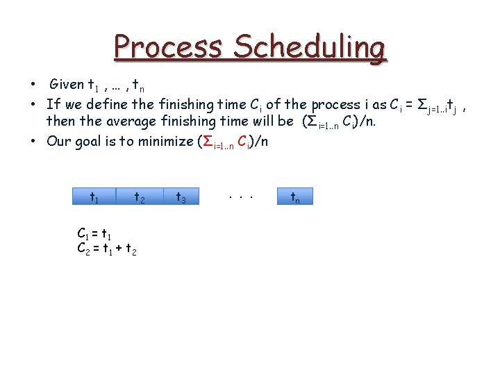
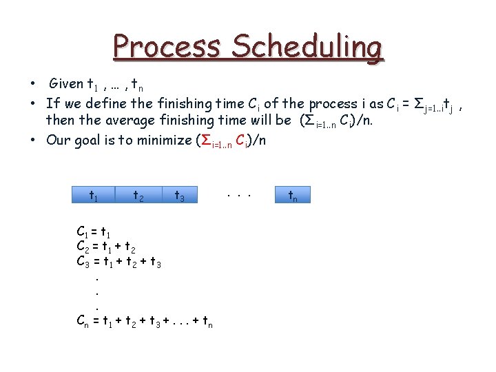
Process Scheduling • Given t 1 , … , tn • If we define the finishing time Ci of the process i as Ci = Σj=1. . itj , then the average finishing time will be (Σi=1. . n Ci)/n. • Our goal is to minimize (Σi=1. . n Ci)/n t 1 t 2 C 1 = t 1 C 2 = t 1 + t 2 t 3 . . . tn

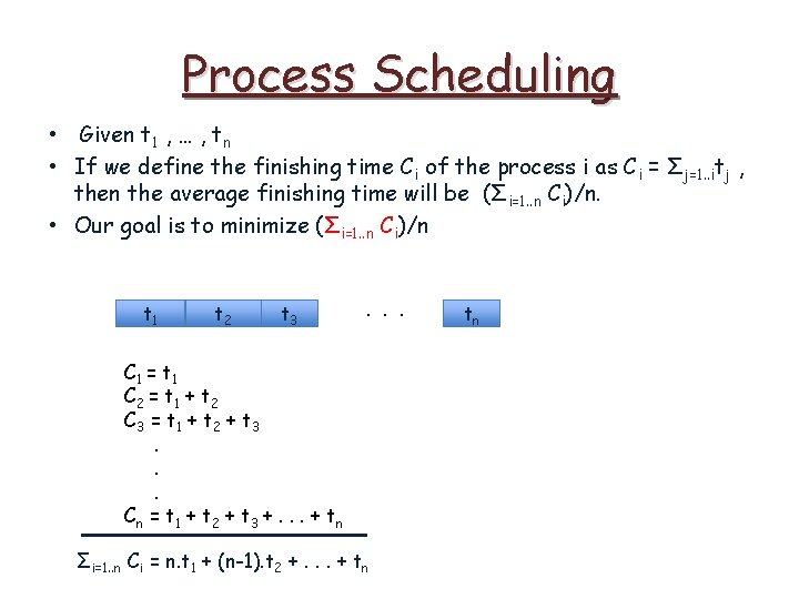
Process Scheduling • Given t 1 , … , tn • If we define the finishing time Ci of the process i as Ci = Σj=1. . itj , then the average finishing time will be (Σi=1. . n Ci)/n. • Our goal is to minimize (Σi=1. . n Ci)/n t 1 t 2 t 3 C 1 = t 1 C 2 = t 1 + t 2 C 3 = t 1 + t 2 + t 3. . . C n = t 1 + t 2 + t 3 +. . . + t n . . . tn

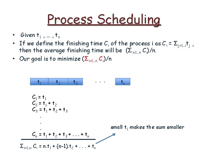
Process Scheduling • Given t 1 , … , tn • If we define the finishing time Ci of the process i as Ci = Σj=1. . itj , then the average finishing time will be (Σi=1. . n Ci)/n. • Our goal is to minimize (Σi=1. . n Ci)/n t 1 t 2 t 3 . . . C 1 = t 1 C 2 = t 1 + t 2 C 3 = t 1 + t 2 + t 3. . . C n = t 1 + t 2 + t 3 +. . . + t n Σi=1. . n Ci = n. t 1 + (n-1). t 2 +. . . + tn tn

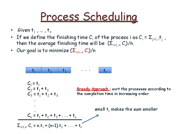
Process Scheduling • Given t 1 , … , tn • If we define the finishing time Ci of the process i as Ci = Σj=1. . itj , then the average finishing time will be (Σi=1. . n Ci)/n. • Our goal is to minimize (Σi=1. . n Ci)/n t 1 t 2 t 3 . . . C 1 = t 1 C 2 = t 1 + t 2 C 3 = t 1 + t 2 + t 3. . . C n = t 1 + t 2 + t 3 +. . . + t n Σi=1. . n Ci = n. t 1 + (n-1). t 2 +. . . + tn tn small t 1 makes the sum smaller

Process Scheduling • Given t 1 , … , tn • If we define the finishing time Ci of the process i as Ci = Σj=1. . itj , then the average finishing time will be (Σi=1. . n Ci)/n. • Our goal is to minimize (Σi=1. . n Ci)/n t 1 t 2 t 3 . . . tn C 1 = t 1 C 2 = t 1 + t 2 Greedy Approach : sort the processes according to the completion time in increasing order C 3 = t 1 + t 2 + t 3. . small t 1 makes the sum smaller. C n = t 1 + t 2 + t 3 +. . . + t n Σi=1. . n Ci = n. t 1 + (n-1). t 2 +. . . + tn

Process Scheduling Theorem (Greedy-choice property): Let S be a sequence of processes ordered according to the completion time. Then S is an optimal sequence. (Our greedy approach yields us an optimal solution) Proof

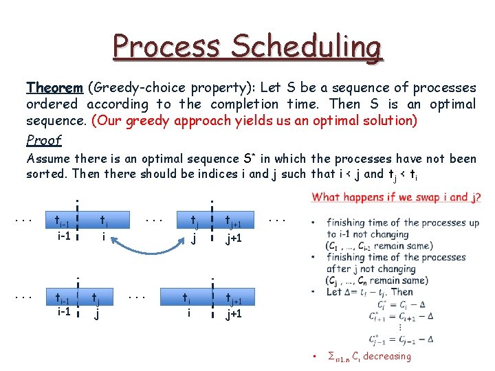
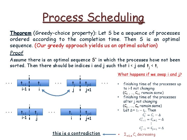
Process Scheduling Theorem (Greedy-choice property): Let S be a sequence of processes ordered according to the completion time. Then S is an optimal sequence. (Our greedy approach yields us an optimal solution) Proof Assume there is an optimal sequence S* in which the processes have not been sorted.

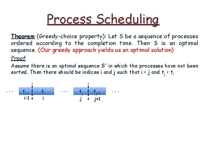
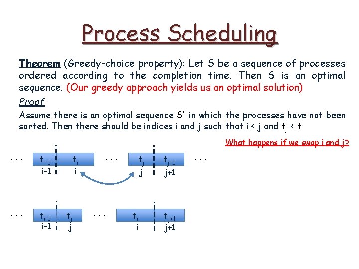
Process Scheduling Theorem (Greedy-choice property): Let S be a sequence of processes ordered according to the completion time. Then S is an optimal sequence. (Our greedy approach yields us an optimal solution) Proof Assume there is an optimal sequence S* in which the processes have not been sorted. Then there should be indices i and j such that i < j and tj < ti. . . ti-1 ti i . . . tj j tj+1 . . .

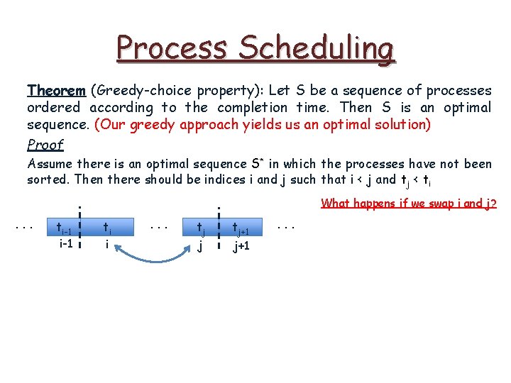
Process Scheduling Theorem (Greedy-choice property): Let S be a sequence of processes ordered according to the completion time. Then S is an optimal sequence. (Our greedy approach yields us an optimal solution) Proof Assume there is an optimal sequence S* in which the processes have not been sorted. Then there should be indices i and j such that i < j and tj < ti What happens if we swap i and j? . . . ti-1 ti i . . . tj j tj+1 . . .

Process Scheduling Theorem (Greedy-choice property): Let S be a sequence of processes ordered according to the completion time. Then S is an optimal sequence. (Our greedy approach yields us an optimal solution) Proof Assume there is an optimal sequence S* in which the processes have not been sorted. Then there should be indices i and j such that i < j and tj < ti What happens if we swap i and j? . . . ti-1 i-1 . . . ti i tj j . . . ti i tj+1 j+1 . . .

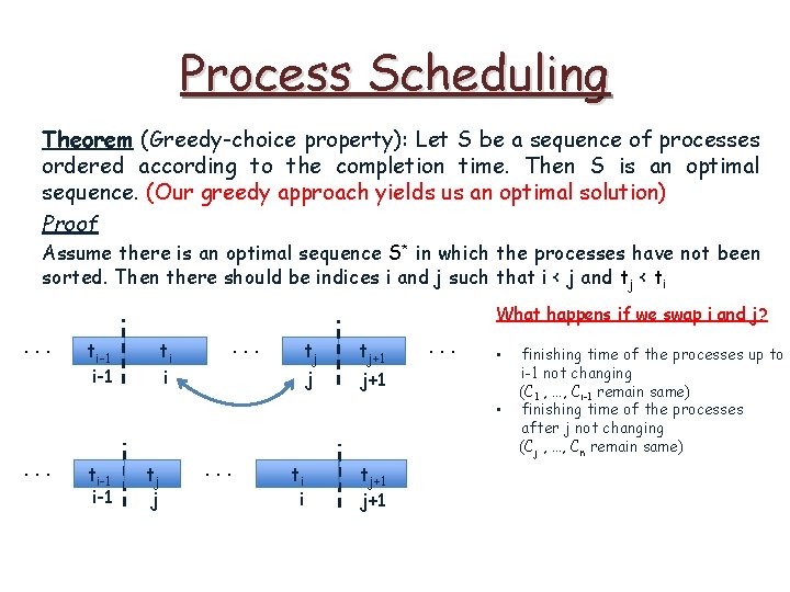
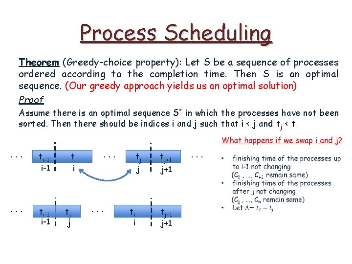
Process Scheduling Theorem (Greedy-choice property): Let S be a sequence of processes ordered according to the completion time. Then S is an optimal sequence. (Our greedy approach yields us an optimal solution) Proof Assume there is an optimal sequence S* in which the processes have not been sorted. Then there should be indices i and j such that i < j and tj < ti What happens if we swap i and j? . . . ti-1 . . . ti i tj j tj+1 . . . • j+1 • . . . ti-1 tj j . . . ti i tj+1 finishing time of the processes up to i-1 not changing (C 1 , …, Ci-1 remain same) finishing time of the processes after j not changing (Cj , …, Cn remain same)

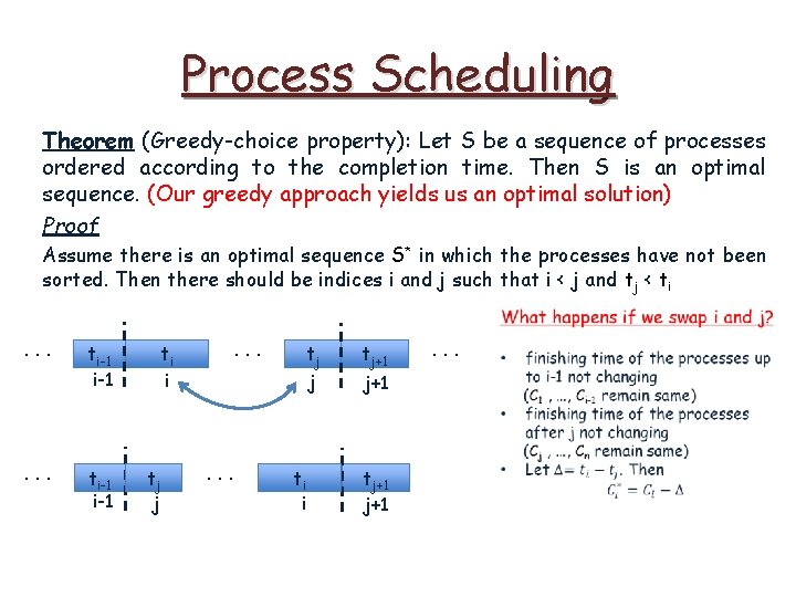
Process Scheduling Theorem (Greedy-choice property): Let S be a sequence of processes ordered according to the completion time. Then S is an optimal sequence. (Our greedy approach yields us an optimal solution) Proof Assume there is an optimal sequence S* in which the processes have not been sorted. Then there should be indices i and j such that i < j and tj < ti . . . ti-1 i-1 . . . ti i tj j . . . ti i tj+1 j+1 . . .

Process Scheduling Theorem (Greedy-choice property): Let S be a sequence of processes ordered according to the completion time. Then S is an optimal sequence. (Our greedy approach yields us an optimal solution) Proof Assume there is an optimal sequence S* in which the processes have not been sorted. Then there should be indices i and j such that i < j and tj < ti . . . ti-1 i-1 . . . ti i tj j . . . ti i tj+1 j+1 . . .

Process Scheduling Theorem (Greedy-choice property): Let S be a sequence of processes ordered according to the completion time. Then S is an optimal sequence. (Our greedy approach yields us an optimal solution) Proof Assume there is an optimal sequence S* in which the processes have not been sorted. Then there should be indices i and j such that i < j and tj < ti . . . ti-1 i-1 . . . ti i tj j . . . ti i tj+1 j+1 . . .

Process Scheduling Theorem (Greedy-choice property): Let S be a sequence of processes ordered according to the completion time. Then S is an optimal sequence. (Our greedy approach yields us an optimal solution) Proof Assume there is an optimal sequence S* in which the processes have not been sorted. Then there should be indices i and j such that i < j and tj < ti . . . ti-1 i-1 . . . ti i tj j . . . ti i tj+1 . . . j+1 tj+1 • Σi=1. . n Ci decreasing

Process Scheduling Theorem (Greedy-choice property): Let S be a sequence of processes ordered according to the completion time. Then S is an optimal sequence. (Our greedy approach yields us an optimal solution) Proof Assume there is an optimal sequence S* in which the processes have not been sorted. Then there should be indices i and j such that i < j and tj < ti . . . ti-1 i-1 . . . ti i tj j . . . ti i tj+1 . . . j+1 tj+1 this is a contradiction • Σi=1. . n Ci decreasing