Greedy Algorithms I Greed for lack of a

Greedy Algorithms (I) Greed, for lack of a better word, is good! Greed is right! Greed works! - Michael Douglas, U. S. actor in the role of Gordon Gecko, in the film Wall Street, 1987

Main topics n n n Idea of the greedy approach Change-making problem Minimum spanning tree problem n n Prim’s algorithm Kruskal’s algorithm Properties of minimum spanning tree (additive part) Bottleneck spanning tree (additive part)

Expected Outcomes n Student should be able to n n n n summarize the idea of the greedy technique list several applications of the greedy technique apply the greedy technique to change-making problem define the minimum spanning tree problem describe ideas of Prim and Kruskal’s algorithms for computing minimum spanning tree prove the correctness of the two algorithms analyze the time complexities of the two algorithms under different data structures prove the various properties of minimum spanning tree

Anticipatory Set: Change Making Problem n n How to make 48 cents of change using coins of denominations of 25 (1 quarter coin), 10 (1 dime coin), 5 (1 nickel coin), and 1 (1 penny coin) so that the total number of coins is the smallest? The idea: n n n Take the coin with largest denomination without exceeding the remaining amount of cents, make the locally best choice at each step. Is the solution optimal? Yes, the proof is left as exercise.

General Change-Making Problem Given unlimited amounts of coins of denominations d 1 > … > dm , give change for amount n with the least number of coins. Does the greedy algorithm always give an optimal solution for the general change-making problem? We give the following example, Example: d 1 = 7 c, d 2 =5 c, d 3 = 1 c, and n = 10 c, not always produces an optimal solution. in fact, for some instances, the problem may not have a solution at all! consider instance d 1 = 7 c, d 2 =5 c, d 3 = 3 c, and n = 11 c. But, this problem can be solved by dynamic programming, please try to design an algorithm for the general change-making problem after class.

Greedy Algorithms n A greedy algorithm makes a locally optimal choice step by step in the hope that this choice will lead to a globally optimal solution. The choice made at each step must be: n Feasible n n locally optimal n n Be the best local choice among all feasible choices Irrevocable n n Satisfy the problem’s constraints Once made, the choice can’t be changed on subsequent steps. Do greedy algorithms always yield optimal solutions? n Example: change making problem with a denomination set of 7, 5 and 1, and n =10?

Applications of the Greedy Strategy For some problems, yields an optimal solution for every instance. For most, does not but can be useful for fast approximations. n Optimal solutions: n n n some instances of change making Minimum Spanning Tree (MST) Single-source shortest paths Huffman codes Approximations: n n n Traveling Salesman Problem (TSP) Knapsack problem other optimization problems

Minimum Spanning Tree (MST) n Spanning tree of a connected graph G is a connected acyclic subgraph (tree) of G that includes all of G’s vertices. n n n Note: a spanning tree with n vertices has exactly n-1 edges. Minimum Spanning Tree of a weighted, connected graph G is a spanning tree of G of minimum total weight. Example:

MST Problem n n Given a connected, undirected, weighted graph G= (V, E), find a minimum spanning tree for it. Compute MST through Brute Force? • Brute force • • • Feasibility of Brute force • n Generate all possible spanning trees for the given graph. Find the one with minimum total weight. Possible too many trees (exponential for dense graphs) Kruskal: 1956, Prim: 1957

The Prim’s Algorithm n n Idea of the Prim’s algorithm Pseudo-code of the algorithm Correctness of the algorithm (important) Time complexity of the algorithm

Idea of Prim n Grow a single tree by repeatedly adding the least cost edge (greedy step) that connects a vertex in the existing tree to a vertex not in the existing tree n Intermediate solution is always a subtree of some minimum spanning tree.

Prim’s MST algorithm n Start with a tree , T 0 , consisting of one vertex n “Grow” tree one vertex/edge at a time Construct a series of expanding subtrees T 1, T 2, … Tn-1. . At each stage construct Ti from Ti-1 by n adding the minimum weight edge that connecting a vertex in tree (Ti-1) to a vertex not yet in the tree n n this is the “greedy” step! Algorithm stops when all vertices are included

Pseudocode of the Prim ALGORITHM Prim(G) //Prim’s algorithm for constructing a minimum spanning tree //Input: A weighted connected graph G = (V, E) //Output: ET, the set of edges composing a minimum spanning tree of G VT {v 0} //v 0 can be arbitrarily selected ET for i 1 to |V|-1 do find a minimum-weight edge e* = (v*, u*) among all the edges (v, u) such that v is in VT and u is in V-VT VT {u*} ET {e*} return ET

An example 5 a c 6 4 1 3 b d 2 7 e

The Prim’s algorithm is greedy! n The choice of edges added to current subtree satisfying the three properties of greedy algorithms. n n n Feasible, each edge added to the tree does not result in a cycle, guarantee that the final ET is a spanning tree Local optimal, each edge selected to the tree is always the one with minimum weight among all the edges crossing VT and V-VT Irrevocable, once an edge is added to the tree, it is not removed in subsequent steps.

Correctness of Prim n Prove by induction that this construction process actually yields MST. n n T 0 is a subset of all MSTs Suppose that Ti-1 is a subset of some MST T, we should prove that Ti which is generated from Ti-1 is also a subset of some MST. n n By contradiction, assume that Ti does not belong to any MST. Let ei = (u, v) be the minimum weight edge from a vertex in Ti-1 to a vertex not in Ti-1 used by Prim’s algorithm to expanding Ti-1 to Ti , according to our assumption, ei can not belong to MST T. Adding ei to T results in a cycle containing another edge e’ = (u’, v’) connecting a vertex u’ in Ti-1 to a vertex v’ not in it, and w(e’) w(ei) according to the greedy Prim’s algorithm. Removing e’ from T and adding ei to T results in another spanning tree T’ with weight w(T’) w(T), indicating that T’ is a minimum spanning tree including Ti which contradict to assumption that Ti does not belong to any MST.

Correctness of Prim

Implementation of Prim n How to implement the steps in the Prim’s algorithm? n n n First idea, label each vertex with either 0 or 1, 1 represents the vertex in VT, and 0 otherwise. Traverse the edge set to find an minimum weight edge whose endpoints have different labels. Time complexity: O(VE) if adjacency linked list and O(V 3) for adjacency matrix n n For sparse graphs, use adjacency linked list Any improvement?

Notations n n T: the expanding subtree. Q: the remaining vertices. At each stage, the key point of expanding the current subtree T is to n Determine which vertex in Q is the nearest vertex to T. n Q can be thought of as a priority queue: n n n The key (priority) of each vertex, key[v], means the minimum weight edge from v to a vertex in T. Key[v] is ∞ if v is not linked to any vertex in T. The major operation is to to find and delete the nearest vertex (v, for which key[v] is the smallest among all the vertices) Remove the nearest vertex v from Q and add it and the corresponding edge to T. n With the occurrence of that action, the key of v’s neighbors will be changed. To remember the edges of the MST, an array [] is introduced to record the parent of each vertex. That is [v] is the vertex in the expanding subtree T that is closest to v not in T.

Advanced Prim’s Algorithm ALGORITHM MST-PRIM( G, w, r ) //w: weight; r: root, the starting vertex 1. 2. 3. 4. 5. 6. 7. 8. 9. 10. 11. for each u V[G] do key[u] NIL // [u] : the parent of u key[r] 0 Q V[G] //Now the priority queue, Q, has been built. while Q do u Extract-Min(Q) //remove the nearest vertex from Q for each v Adj[u] // update the key for each of v’s adjacent nodes. do if v Q and w(u, v) < key[v] then [v] u key[v] w(u, v)

Time Complexity of Prim’s algorithm n Need priority queue for locating the nearest vertex n n Use unordered array to store the priority queue: Efficiency: Θ(n 2) Use binary min-heap to store the priority queue Efficiency: For graph with n vertices and m edges: O(m log n) n Use Fibonacci-heap to store the priority queue: Efficiency: For graph with n vertices and m edges: O(n log n + m)

Kruskal’s MST Algorithm n n n Edges are initially sorted by increasing weight Start with an empty forest F 0 “grow” MST one edge at a time through a series of expanding forests F 1, F 2, …, Fn-1 n intermediate stages usually have forest of trees (not connected) n n at each stage add minimum weight edge among those not yet used that does not create a cycle n need efficient way of detecting/avoiding cycles algorithm stops when all vertices are included

Correctness of Kruskal n n Similar to the proof of Prim Prove by induction on the construction process actually generate a MST n Consider F 0, F 1, …, Fn-1

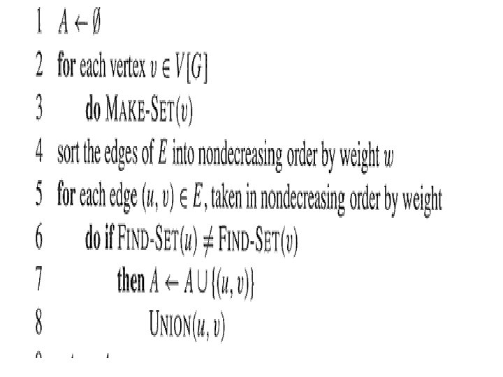
Basic Kruskal’s Algorithm ALGORITHM Kruscal(G) //Input: A weighted connected graph G = <V, E> //Output: ET, the set of edges composing a minimum spanning tree of G. Sort E in nondecreasing order of the edge weights w(ei 1) <= … <= w(ei|E|) ET ; ecounter 0 //initialize the set of tree edges and its size k 0 while encounter < |V| - 1 do k k+1 if ET U {eik} is acyclic ET U {eik} ; ecounter + 1 return ET

Kruskal’s Algorithm (Advanced Part)

Kruskal: Time Complexity 1. O(EV) when disjoint-set data structure are not used. 2. When use disjoint-set data structure with union-by-rank and pathcompression heuristics: a) Initializing the set A in line 1 takes O(1) time. b) O(V) MAKE-SET operations in lines 2 -3 c) Sort the edges in line 4 takes O(Elog. E) time. d) The for loop of lines 5 -8 performs O(E) FIND-SET and UNION operations on the disjoint-set forest − b) and d) take a total of O((V+E) (V)) − Line 9: O(V+E) Note that: E V-1 and (V) = O(log. E) and E V 2 SO total time is: O(Elog. V)

Properties of MST n Property 1: n Let (u, v) be a minimum-weight edge in a graph G = (V, E), then (u, v) belongs to some minimum spanning tree of G. n Proof hint: suppose (u, v) is not in MST T, construct another MST T’ including (u, v).

Properties of MST n Property 2 n n A graph has a unique minimum spanning tree if all the edge weights are pairwise distinct. The converse does not hold.

Properties of MST n Property 3 n n Let T be a minimum spanning tree of a graph G, and let T’ be an arbitrary spanning tree of G, suppose the edges of each tree are sorted in non-decreasing order, that is, w(e 1) w(e 2) … w(en-1) and w(e 1’) w(e 2’) … w(en-1’), then for 1 i n-1, w(ei) w(ei’). Property 4 n Let T be a minimum spanning tree of a graph G, and let L be the sorted list of the edge weights of T, then for any other minimum spanning tree T’ of G, the list L is also the sorted list of edge weights of T’.

Properties of MST n n n Property 5 Let e=(u, v) be a maximum-weight edge on some cycle of G. Prove that there is a minimum spanning tree that does not include e. Proof. Arbitrarily choose a MST T. If T does not contain e, it is proved. Otherwise, Te is disconnected, and suppose X, Y are the two connected components of Te. Let e is on cycle C in G. Let P=Ce. Then there is an edge (x, y) on P such that x X, and y Y. And w(x, y) w(e). T’=Te+(x, y) is a spanning tree and w(T’) w(T). Also we have w(T) w(T’), so w(T’) = w(T). T’ is a MST not including e.

Bottleneck Spanning Tree n A bottleneck spanning tree T of a connected, weighted and undirected graph G is a spanning tree of G whose largest edge weight is minimum over all spanning trees of G. n Let T 1, T 2, …, Tm are all the spanning trees of G, and the largest edge of each tree is et 1, et 2, …, etm, suppose w(eti) w(etj) for 1 j m and j i, then Ti is a bottleneck spanning tree. n The value of a BST T is the weight of the maximumweight edge in T. n The bottleneck spanning tree may not be unique.

BST vs MST n Every minimum spanning tree is a bottleneck spanning tree. n n Property 4 implies it. An easier proof: Let T be a MST and T’ be a BST, let the maximumweight edge in T and T’ be e and e’, respectively. Suppose for the contrary that the MST T is not a BST, then we have w(e)>w(e’), which also indicates that the weight of e is greater than that of any edges in T’. Removing e from T disconnects T into two subtrees T 1 and T 2, there must exist an edge f in T’ connecting T 1 and T 2, otherwise, T is not connected. T 1 T 2 {f} forms a new tree T’’ with w(T’’) = w(T) - w(e) + w(f) < w(T), A contradiction to the fact that T is MST, thus, A MST is also a BST.

Shortest Paths – Dijkstra’s Algorithm n Shortest Path Problems n n All pair shortest paths (Floy’s algorithm) Single Source Shortest Paths Problem (Dijkstra’s algorithm): Given a weighted graph G, find the shortest paths from a source vertex s to each of the other vertices. 4 a c 5 2 3 7 b d 6 4 e

3 a Tree vertices a(-, 0) b(a, 3) 4 b 7 2 c 5 d 4 6 e Remaining vertices b(a, 3) c(-, ∞) d(a, 7) e(-, ∞) 3 a c(b, 3+4) d(b, 3+2) e(-, ∞) 3 c(b, 7) e(d, 5+4) e(d, 9) a e(d, 9) 6 5 c 6 5 d e 4 4 2 7 c d b e 4 4 7 6 5 2 3 c d b a c(b, 7) 2 7 a d(b, 5) 4 b 4 e

Prim’s and Dijkstra’s Algorithms n Generate different kinds of spanning trees n n n Different greedy strategies n n n Prim’s: a minimum spanning tree. Dijkstra’s : a spanning tree rooted at a given source s, such that the distance from s to every other vertex is the shortest. Prims’: Always choose the closest (to the tree) vertex in the priority queue Q to add to the expanding tree VT. Dijkstra’s : Always choose the closest (to the source) vertex in the priority queue Q to add to the expanding tree VT. Different labels for each vertex n n Prims’: parent vertex and the distance from the tree to the vertex. . Dijkstra’s : parent vertex and the distance from the source to the vertex.

Shortest Paths-Dijkstra’s Algorithm n Dijkstra’s algorithm: Similar to Prim’s MST algorithm, with the following difference: n Start with tree consisting of one vertex. n n “Grow” tree one vertex/edge at a time. n Construct a series of expanding subtrees T 1, T 2, … Keep track of shortest path from source to each of the vertices in T i At each stage construct Ti+1 from Ti: add minimum weight edge connecting a vertex in tree (Ti) to one not yet in tree n choose from “fringe” edges n (this is the “greedy” step!) edge (u*, u) with lowest du* + w(u*, u) Algorithm stops when all vertices are included.

Dijkstra’s Algorithm ALGORITHM Dijkstra(G, s) //Input: A weighted connected graph G = <V, E> and a source vertex s //Output: The length dv of a shortest path from s to v and its penultimate vertex pv for every vertex v in V Initialize (Q) for every vertex v in V do dv ∞ ; Pv null insert(Q, v, dv) //initialize vertex priority in the priority queue ds 0; Decrease(Q, s, ds) VT //update priority of s with ds, making ds, the minimum for i 0 to |V| - 1 do // Pv , the parent of v //initialize vertex priority in the priority queue //produce |V| - 1 edges for the tree u* Delete. Min(Q) //delete the minimum priority element VT VT U {u*} //expanding the tree, choosing the locally best vertex for every vertex u in V – VT that is adjacent to u* do if du* + w(u*, u) < du du + w(u*, u); pu u* Decrease(Q, u, du)

Correctness of Dijkstra’s n n Dijkstra’s algorithm, run on a weighted, directed graph G=(V, E), with non-negative weight function w and source s, terminates with d[u]= (s, u) for all vertices u V. Here (s, u) means the shortest distance from s to u. Proof (by contradiction) n Since S = V in the end and for each vertex v, after it was put into S, the value of d[u] would never be changed. we only need to prove that for each vertex v added to S, there holds d[v]= (s, v) when v is added to S. n Suppose that u is the first vertex for which d[u] (s, u) when it was added to S n Note n u is not s because d[s] = 0= d(s, s) n There must be a path s. . . u, since otherwise d[u]= (s, u) = . n Since there’s a path, there must be a shortest path (note there is no negative cycle).

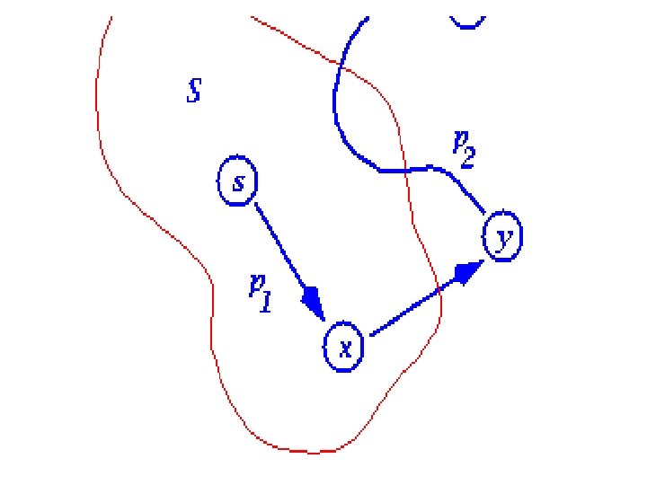
Dijkstra’s Algorithm - Proof n n n Let s®x®y®u be the shortest path from s to u, where at the moment u is chosen to S, x is in S and y is the first outside S (y may not exist) When x was added to S, d[x] = d(s, x) Edge x®y will be considered at that time, d[y] <= d(s, x)+w(x, y) = d(s, y) (why? )

Dijkstra’s Algorithm - Proof n n n n so d[y] = d ( s , y) d( s , u ) d [ u ] But, when we chose u, both u and y are in Q, so d[u] d[y] (otherwise we would have chosen y) Thus the inequalities must be equalities d [ y] = d ( s , y) = d ( s , u ) = d [ u ] And our hypothesis (d[u] d(s, u)) is contradicted! Note! if such y does not exist, proof is easier

Notes on Dijkstra’s Algorithm n Doesn’t work with negative weights n n Can you give a counter example? How about if the negative weight edges are from s? Applicable to both undirected and directed graphs Efficiency n Use unordered array to store the priority queue: Θ(n 2) n Use min-heap to store the priority queue: n Use Fibonacci-heap, O(nlog n+m) O(m log n)

Bellman’s Algorithm Negative weight edge is permitted!

Linear Programming n Linear programming problem: n n n Input: matrix Amn, vector bm, and vector cn. Output: vector xn, such that maximize c. Tx subject to Ax b. Notes n n This problem has polynomial time solution. Many problems can be reduced to LP.

Feasibility Problem of LP n n Feasible solution: xn, subject to Ax b. Feasibility problem of LP: n n Given A, b, c Output: either a feasible solution x if one exists, or a judgment that no feasible solution exists.

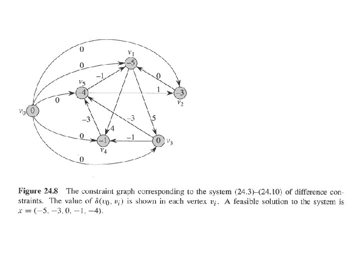
Systems of difference constraints n n Each row of A contains exactly one “ 1” and one “-1”. All other elements are “ 0”. Each row is a difference constraint: x -x 0 x -x -1 n xj-xi bk, 1 k m. x -x 1 An example x -x 5 1 2 1 5 2 - n 3 5 1 x 4 -x 1 4 x 4 -x 3 -1 x 5 -x 3 -3 n x 5 -x 4 -3 Solution x = (-5, -3, 0, -1, -4); x’=(-5+d, -3+d, 0+d, -1+d, -4+d)

Constraints graph n n Given a system Ax b of difference constraints The constraint graph is a weighted, directed graph G = (V, E; W), where: n V={v 0, v 1, …, vn} //v 0 is an extra vertex n E={(vi, vj): xj-xi bk is a constraint} {(v 0, v 1), (v 0, v 2), …, (v 0, vn)}. //each vertex is reachable from v 0 n w(vi, vj) = bk, if xj-xi bk is a constraint; n w(v 0, vi) = 0.

Constraint graph of example

Solve Difference Constraints by SSSP in constraint graph n Given a system Ax b of difference constraints, let G = (V, E; W) be the corresponding constraint graph. 1. If G contains no negative-weight cycles, then x = ( (v 0, v 1), (v 0, v 2), …, (v 0, vn)) is a feasible solution for the system. 2. If G contains a negative-weight cycle, then there is no feasible solution for the system.

Solution to Difference Constraints n n Bellman-Ford algorithm. If G contains no negative-weight cycle, then, it contains no negative-weight cycle reachable from v 0, then Bellman-Ford returns TRUE, and x = ( (v 0, v 1), …, (v 0, vn)) gives a solution. If G contains a negative-weight cycle, then this cycle must be reachable from v 0. Then Bellman. Ford returns FALSE. Time complexity: O(VE) = O((n+1)(n+m)) = O(n 2+nm)