Graylevel images Image thresholding During the thresholding process

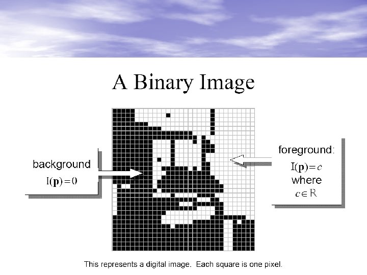
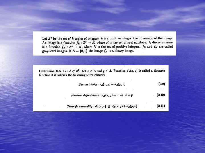
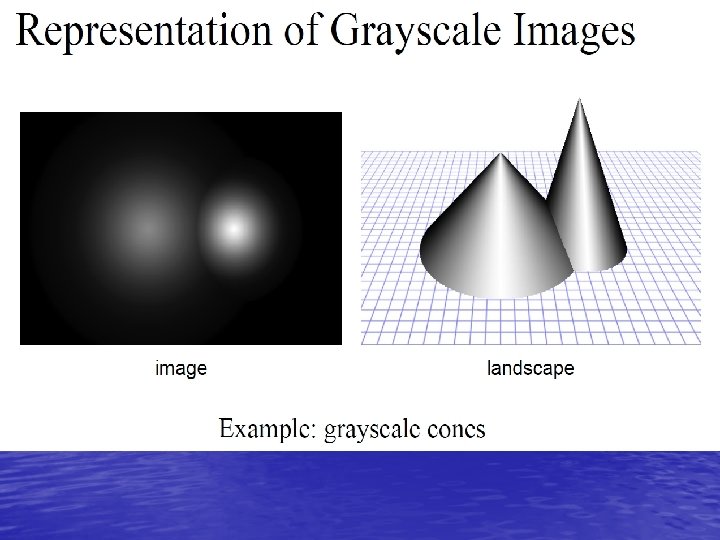
Gray-level images

Image thresholding During the thresholding process, individual pixels in an image are marked as “object” pixels if their value is greater than some threshold value (assuming an object to be brighter than the background) and as “background” pixels otherwise. This convention is known as threshold above. Variants include threshold below, which is opposite of threshold above; threshold inside, where a pixel is labeled "object" if its value is between two thresholds; and threshold outside, which is the opposite of threshold inside (Shapiro, et al. 2001: 83). Typically, an object pixel is given a value of “ 1” while a background pixel is given a value of “ 0. ” Finally, a binary image is created by coloring each pixel white or black, depending on a pixel's label.

Image thresholding Sezgin and Sankur (2004) categorize thresholding methods into the following six groups based on the information the algorithm manipulates (Sezgin et al. , 2004): • histogram shape-based methods, where, for example, the peaks, valleys and curvatures of the smoothed histogram are analyzed • clustering-based methods, where the gray-level samples are clustered in two parts as background and foreground (object), or alternately are modeled as a mixture of two Gaussians • entropy-based methods result in algorithms that use the entropy of the foreground and background regions, the cross-entropy between the original and binarized image, etc. • object attribute-based methods search a measure of similarity between the gray-level and the binarized images, such as fuzzy shape similarity, edge coincidence, etc. • spatial methods [that] use higher-order probability distribution and/or correlation between pixels • local methods adapt the threshold value on each pixel to the local image characteristics. "

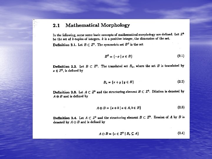
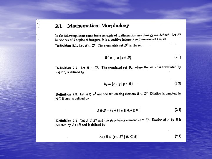
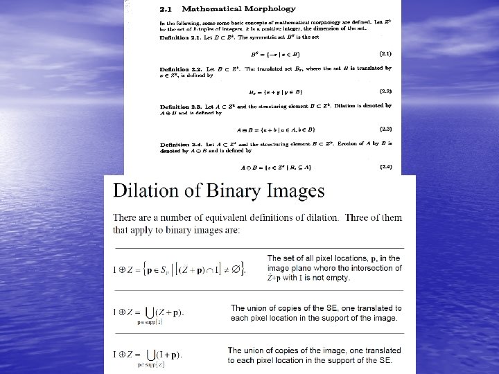
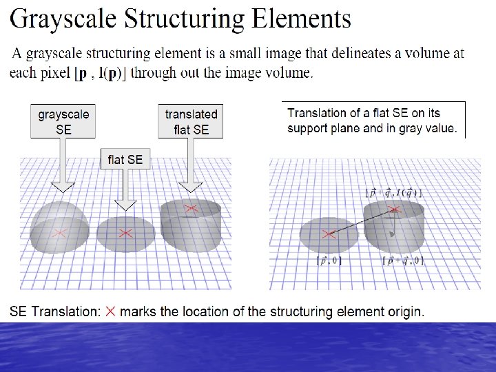
Mathematical morphology • Mathematical Morphology was born in 1964 from the collaborative work of Georges Matheron and Jean Serra, at the École des Mines de Paris, France. • • Matheron supervised the Ph. D thesis of Serra, devoted to the quantification of mineral characteristics from thin cross sections, and this work resulted in a novel practical approach, as well as theoretical advancements in integral geometry and topology.

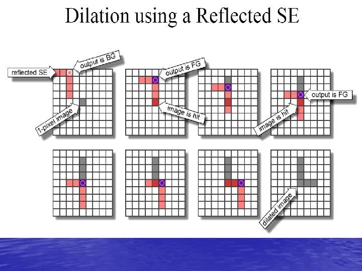
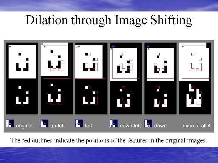
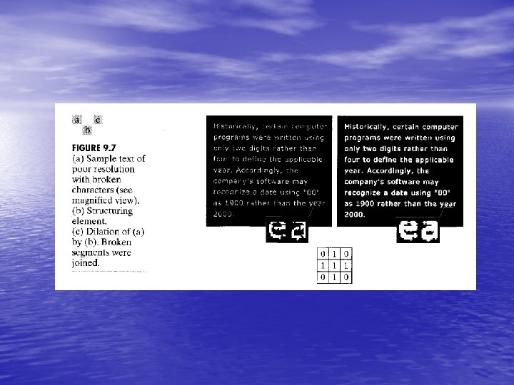
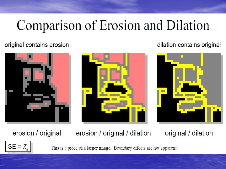
• In 1968, the Centre de Morphologie Mathématique was founded by the École des Mines de Paris in Fontainebleau, France, lead by Matheron and Serra. • During the rest of the 1960's and most of the 1970's, MM dealt essentially with binary images, treated as sets, and generated a large number of binary operators and techniques: Hit-or-miss transform, dilation, erosion, opening, closing, granulometry, thinning, skeletonization, ultimate erosion, conditional bisector, and others. • A random approach was also developed, based on novel image models. Most of the work in that period was developed in Fontainebleau. • The name ‘Mathematical Morphology’ for the new discipline was coined in a pub.

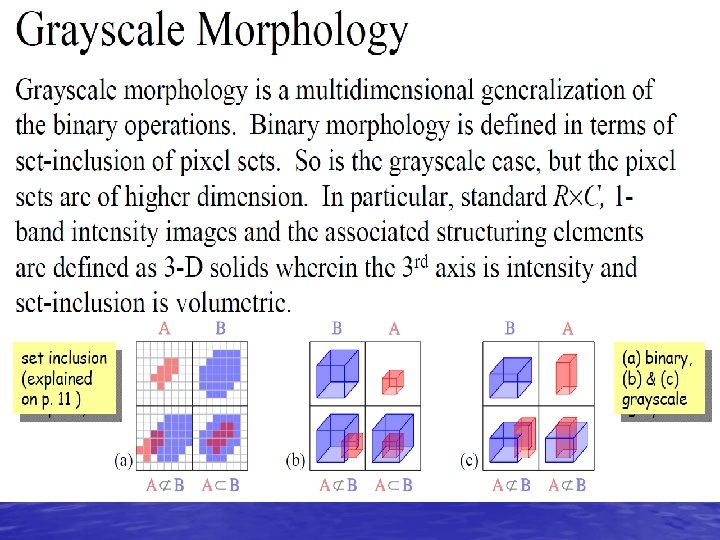
• From mid-1970's to mid-1980's, MM was generalized to grayscale functions and images as well. • Besides extending the main concepts (such as dilation, erosion, etc. . . ) to functions, this generalization yielded new operators, such as morphological gradients, top-hat transform and the Watershed (MM's main segmentation approach). • In the 1980's and 1990's, MM gained a wider recognition, as research centers in several countries began to adopt and investigate the method. • MM started to be applied to a large number of imaging problems and applications.

• In 1986, Jean Serra further generalized MM, this time to a theoretical framework based on complete lattices. • This generalization brought flexibility to theory, enabling its application to a much larger number of structures, including color images, video, graphs, meshes, etc. . . • At the same time, Matheron and Serra also formulated a theory for morphological filtering, based on the new lattice framework. • The 1990's and 2000's also saw further theoretical advancements, including the concepts of connections and levelings.

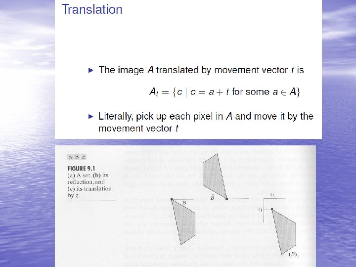
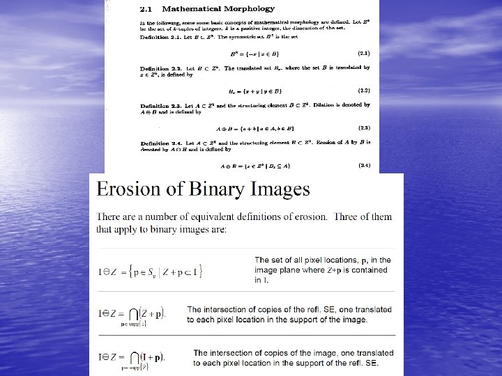
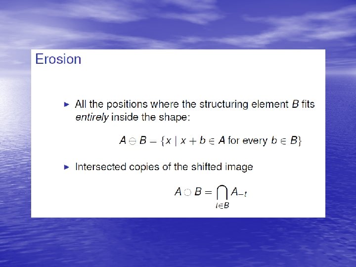
When the structuring element B has a center (e. g. , B is a disk or a square), and this center is located on the origin of E, then the erosion of A by B can be understood as the locus of points reached by the center of B when B moves inside A.

Erosion and dilation in Matlab

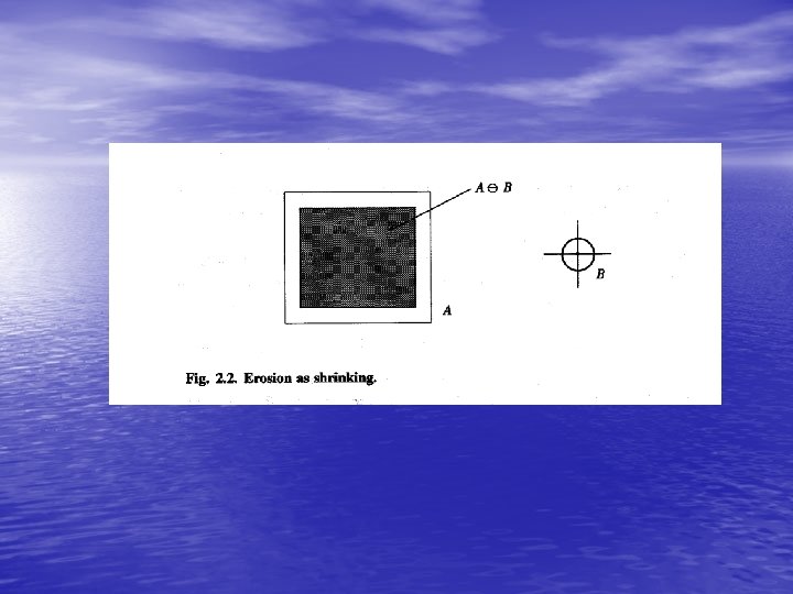
The erosion of the dark-blue square by a disk, resulting in the light-blue square.

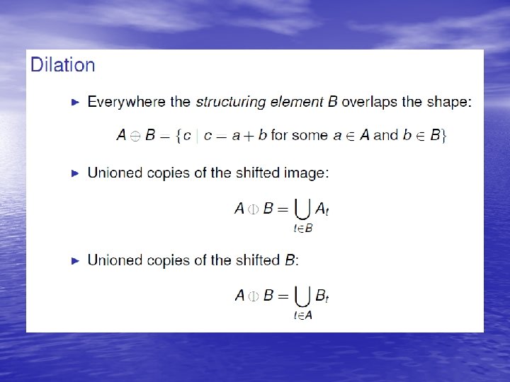
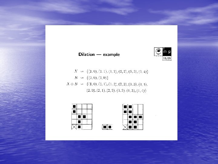
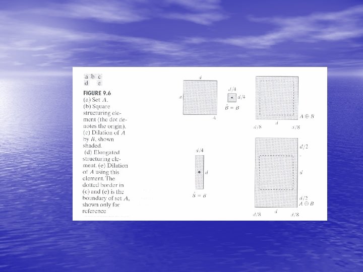
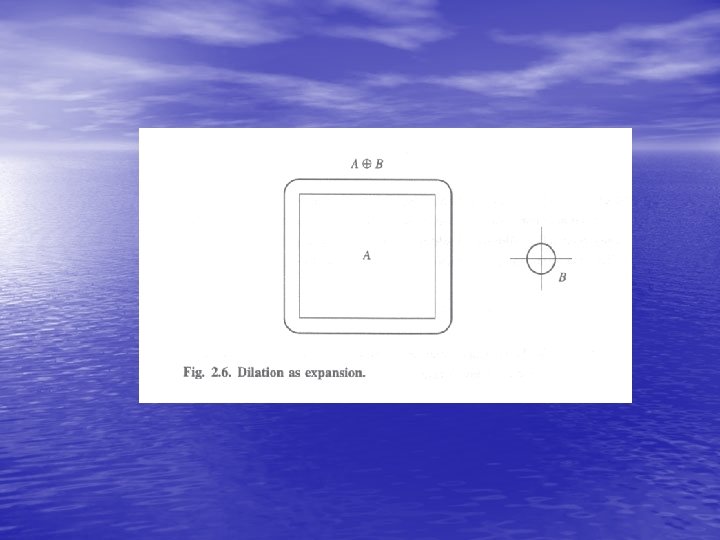
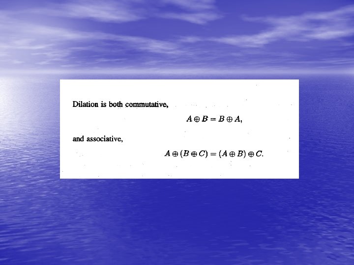
Dilation Alternative way to "see it"

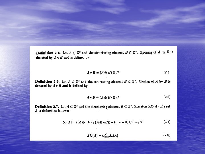
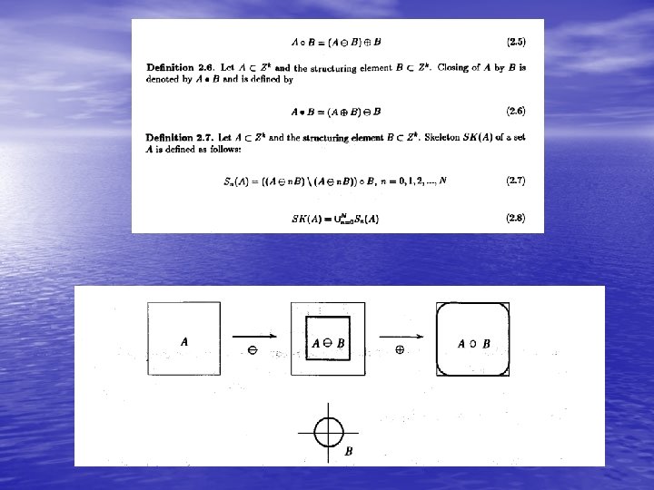
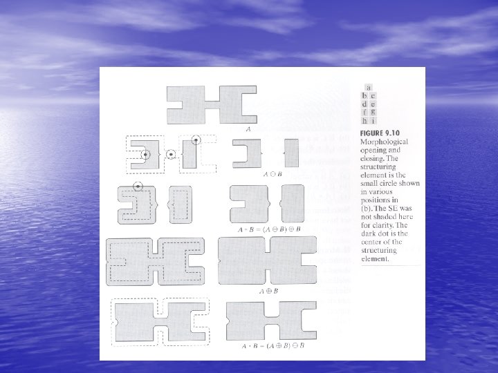
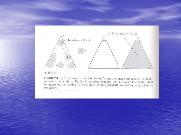
Opening

Opening Alternative way to "see it"

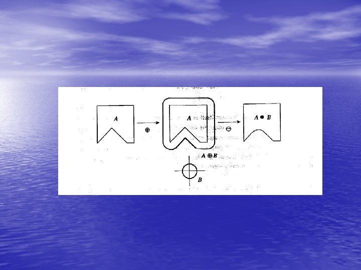
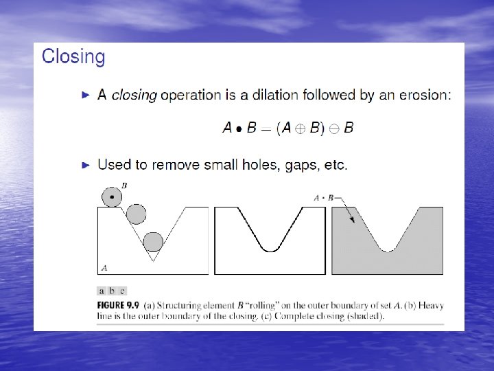
Closing

Grayscale Dilation • Grayscale Dilation: A grayscale image F dilated by a grayscale SE K is defined as: • It generally brighten the source image.

Grayscale Dilation • Bright regions surrounded by dark regions grow in size • Dark regions surrounded by bright regions shrink in size. • Small dark spots in images will disappear as they get `filled in' to the surrounding intensity value. • Small bright spots will become larger spots. • The effect is most marked at places in the image where the intensity changes rapidly and regions of fairly uniform intensity will be largely unchanged except at their edges.

Grayscale Dilation Matlab code function [out] = graydil(im, se) if (~isa(se, 'strel')) se=strel(se); end seq=getsequence(se); lunghezza=size(seq, 1); out=gdil(im, getnhood(seq(1)), 2); for ii=2: lunghezza out=gdil(out, getnhood(seq(ii)), 2); end

Grayscale Dilation dilation over original

Grayscale Dilation Source image Dilated image

Grayscale Erosion • Grayscale Erosion: A grayscale image F eroded by a grayscale SE K is defined as: • It generally darken the image.

Grayscale Erosion • Bright regions surrounded by dark regions shrink in size • Dark regions surrounded by bright regions grow in size. • Small bright spots in images will disappear as they get eroded away down to the surrounding intensity value • Small dark spots will become larger spots. • The effect is most marked at places in the image where the intensity changes rapidly, and regions of fairly uniform intensity will be left more or less unchanged except at their edges.

Grayscale Erosion Matlab code function [out] = grayero(im, se) if (~isa(se, 'strel')) se=strel(se); end seq=getsequence(se); lunghezza=size(seq, 1); out=gerod(im, getnhood(seq(1)), 2); for ii=2: lunghezza out=gerod(out, getnhood(seq(ii)), 2); end

Grayscale Erosion erosion under original

Grayscale Erosion Source image Eroded image

Grayscale Opening • Grayscale Opening: A grayscale image F opened by a grayscale SE K is defined as: • It can be used to select and preserve particular intensity patterns while attenuating others intensity Width of Opening kernel scan line intensity scan line

Grayscale Opening opened & original

Grayscale Opening Source image Opened image

Grayscale Closing • Grayscale Closing: A grayscale image F closed by a grayscale SE K is defined as: • It is another way to select and preserve particular intensity patterns while attenuating others. intensity Width of closing kernel intensity scan line

Grayscale Closing closing & original

Grayscale Closing Source image Closed image

Grayscale Dilation and Erosion Grayscale dilation and erosion with disk‐shaped structuring elements of radius r = 2. 5, 5. 0, 10. 0

Grayscale Dilation and Erosion Grayscale dilation and erosion with various free‐form structuring elements

Grayscale Opening and Closing Grayscale opening and closing with disk‐shaped structuring elements of radius r = 2. 5, 5. 0, 10. 0

Morphological Edge Detection • Morphological Edge Detection is based on Binary Dilation, Binary Erosion and Image Subtraction. • Morphological Edge Detection Algorithms: – Standard: – External: – Internal:

Morphological Edge Detection F K F K

Morphological Edge Detection F

Morphological Gradient is calculated by grayscale dilation and grayscale Erosion. v It is quite similar to the standard edge detection v We also have external and internal gradient

Morphological Gradient Standar d External Internal

Morphological Smoothing • Morphological Smoothing is based on the observation that a grayscale opening smoothes a grayscale image from above the brightness surface and the grayscale closing smoothes from below. So we could get both smooth like:

Morphological Smoothing

Operators In Software VTK: Ø vtk. Image. Continuous. Dilate 3 D() Ø vtk. Image. Continuous. Erode 3 D() ITK: Ø itk. Grayscale. Dilate. Image. Filter() (Flat SE) Ø itk. Grayscale. Erode. Image. Filter() (Flat SE) Ø itk. Grayscale. Function. Dilate. Image. Filter() (Grayscale SE) Ø itk. Grayscale. Function. Erode. Image. Filter() (Grayscale SE) MATLAB: Ø mmdil(), mmero(), mmopen(), mmclose(), mmgradm()

Top-hat Transform • Top-hat Transform (TT): An efficient segmentation tool for extracting bright (respectively dark) objects from uneven background. v White Top-hat Transform (WTT): (ri is the scalar of SE) v Black Top-hat Transform (BTT):

Top-hat Transform tophat + opened = original tophat: original - opening

Top-hat Transform BTT WTT

Top-hat Transform BTT WTT

Application 1 Detecting runways in satellite airport imagery Source Detect long feature WTT Reconstruction Threshold Final result

The End