Gravity Modeling Theory Presented at the 2016 International

Gravity Modeling Theory Presented at the 2016 International Store Location Conference by Jim Puffer

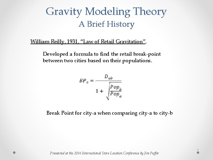
Gravity Modeling Theory A Brief History William Reilly, 1931, “Law of Retail Gravitation”. Developed a formula to find the retail break-point between two cities based on their populations. Break Point for city-a when comparing city-a to city-b Presented at the 2016 International Store Location Conference by Jim Puffer ●

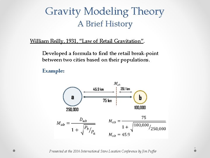
Gravity Modeling Theory A Brief History William Reilly, 1931, “Law of Retail Gravitation”. Developed a formula to find the retail break-point between two cities based on their populations. Example: Presented at the 2016 International Store Location Conference by Jim Puffer ●

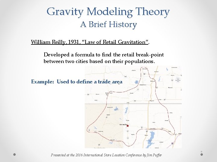
Gravity Modeling Theory A Brief History William Reilly, 1931, “Law of Retail Gravitation”. Developed a formula to find the retail break-point between two cities based on their populations. Example: Used to define a trade area Presented at the 2016 International Store Location Conference by Jim Puffer ●

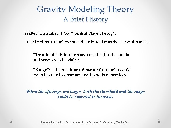
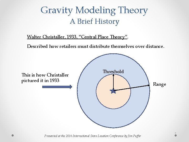
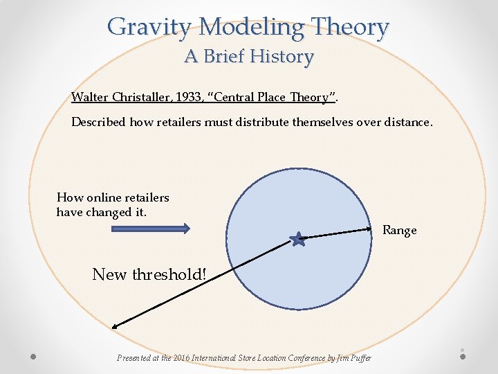
Gravity Modeling Theory A Brief History Walter Christaller, 1933, “Central Place Theory”. Described how retailers must distribute themselves over distance. “Threshold”: Minimum area needed for the goods and services to be viable. “Range”: The maximum distance the retailer could expect to reach consumers with goods or services. When the offerings are larger, both the threshold and the range could be expected to increase. Presented at the 2016 International Store Location Conference by Jim Puffer ●

Gravity Modeling Theory A Brief History Walter Christaller, 1933, “Central Place Theory”. Described how retailers must distribute themselves over distance. This is how Christaller pictured it in 1933 Threshold Presented at the 2016 International Store Location Conference by Jim Puffer Range ●

Gravity Modeling Theory A Brief History Walter Christaller, 1933, “Central Place Theory”. Described how retailers must distribute themselves over distance. How online retailers have changed it. Range New threshold! Presented at the 2016 International Store Location Conference by Jim Puffer ●

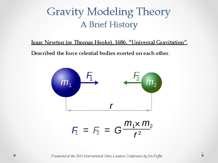
Gravity Modeling Theory A Brief History Isaac Newton (or Thomas Hooke), 1686, “Universal Gravitation”. Described the force celestial bodies exerted on each other. Presented at the 2016 International Store Location Conference by Jim Puffer ●

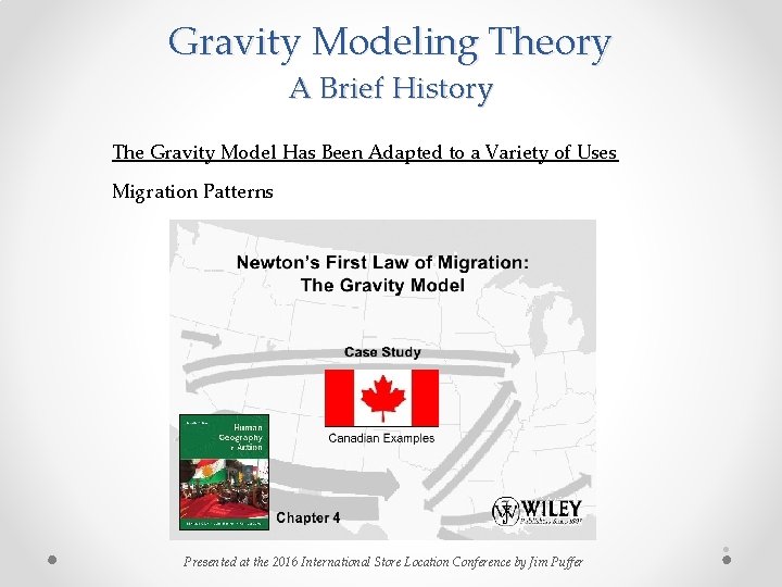
Gravity Modeling Theory A Brief History The Gravity Model Has Been Adapted to a Variety of Uses Migration Patterns Presented at the 2016 International Store Location Conference by Jim Puffer ●

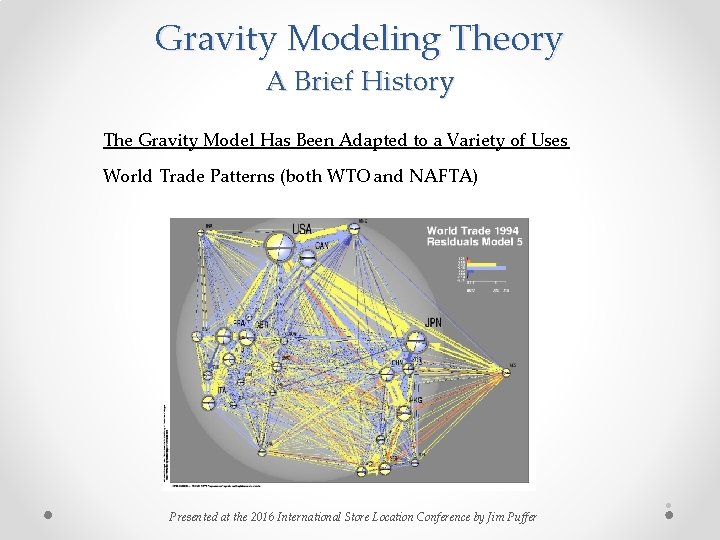
Gravity Modeling Theory A Brief History The Gravity Model Has Been Adapted to a Variety of Uses World Trade Patterns (both WTO and NAFTA) Presented at the 2016 International Store Location Conference by Jim Puffer ●

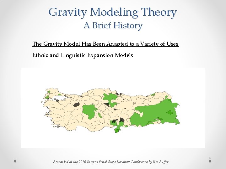
Gravity Modeling Theory A Brief History The Gravity Model Has Been Adapted to a Variety of Uses Ethnic and Linguistic Expansion Models Presented at the 2016 International Store Location Conference by Jim Puffer ●

Gravity Modeling Theory A Brief History The Gravity Model Has Been Adapted to a Variety of Uses ? ? ? ? Presented at the 2016 International Store Location Conference by Jim Puffer ●

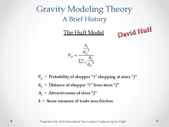
Gravity Modeling Theory A Brief History The Huff Model f f u H d Davi Pij = Probability of shopper “i” shopping at store “j” dij = Distance of shopper “i” from store “j” Aj = Attractiveness of store “j” λ = Some measure of trade area friction Presented at the 2016 International Store Location Conference by Jim Puffer ●

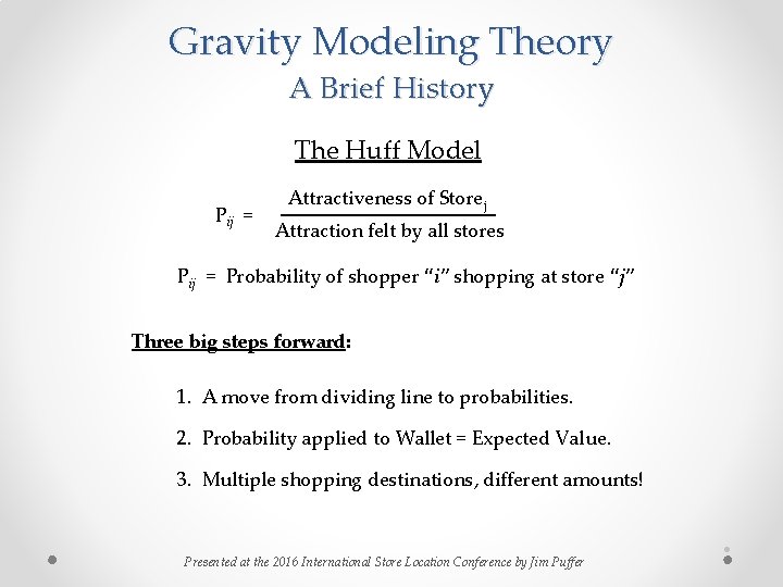
Gravity Modeling Theory A Brief History The Huff Model Pij = Attractiveness of Storej Attraction felt by all stores Pij = Probability of shopper “i” shopping at store “j” Three big steps forward: 1. A move from dividing line to probabilities. 2. Probability applied to Wallet = Expected Value. 3. Multiple shopping destinations, different amounts! Presented at the 2016 International Store Location Conference by Jim Puffer ●

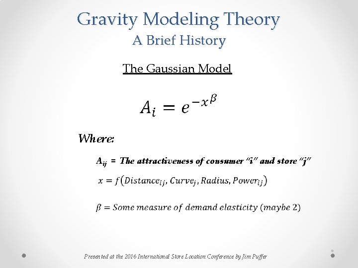
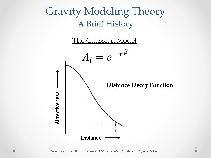
Gravity Modeling Theory A Brief History The Gaussian Model Where: Aij = The attractiveness of consumer “i” and store “j” Presented at the 2016 International Store Location Conference by Jim Puffer ●

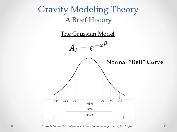
Gravity Modeling Theory A Brief History The Gaussian Model Normal “Bell” Curve Presented at the 2016 International Store Location Conference by Jim Puffer ●

Gravity Modeling Theory A Brief History The Gaussian Model Attractiveness Distance Decay Function Distance Presented at the 2016 International Store Location Conference by Jim Puffer ●

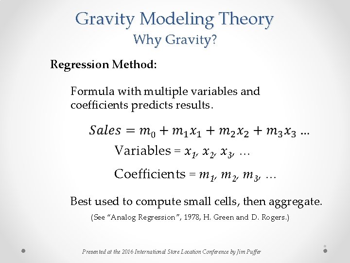
Gravity Modeling Theory Why Gravity? Regression Method: Formula with multiple variables and coefficients predicts results. Variables = x 1, x 2, x 3, … Coefficients = m 1, m 2, m 3, … Best used to compute small cells, then aggregate. (See “Analog Regression”, 1978, H. Green and D. Rogers. ) Presented at the 2016 International Store Location Conference by Jim Puffer ●

Gravity Modeling Theory Why Gravity? Regression Method: Disadvantages Difficult to simulate curves. Tendency towards extreme values. (Disaggregation may help. ) Little room for analyst judgement. Coefficients probably change with T. A. Heterogeneity of sample stores. Autocorrelation cause serious trouble. Presented at the 2016 International Store Location Conference by Jim Puffer ●

Gravity Modeling Theory Why Gravity? Analog Method: m u a b e l l App Bil Use historic data (spotting? ) to predict sales by matching conditions. ● Surrounding competition ● Surrounding population / demographics ● Store format and size Use Excel to build a spreadsheet of smaller areas and analog forecasts, then sum. Presented at the 2016 International Store Location Conference by Jim Puffer ●

Gravity Modeling Theory Why Gravity? Analog Method: Disadvantages Match is never exact How to handle new sizes and formats? New trade areas? New competition? Harder to predict impacts Great for reality checks! Presented at the 2016 International Store Location Conference by Jim Puffer ●

Gravity Modeling Theory Why Gravity? Gravity Method: Advantages Non-linear, matches spotting data Closed monetary system We know where money comes from Shows changes to all stores Works with complicated scenarios Model conditions can be changed quickly Presented at the 2016 International Store Location Conference by Jim Puffer ●

Gravity Modeling Theory Where Do Gravity Models Work? Destination-type trips, returning home Grocery, liquor, scripts, hardware Where accurate competitive sales can be obtained Closed system demands an accurate pool Where accurate per-capita expenditures can be estimated BLS Annual Consumer Expenditure Study Where perceived distances can be measured Distance, drive-time, walk-time, bicycle-time Presented at the 2016 International Store Location Conference by Jim Puffer ●

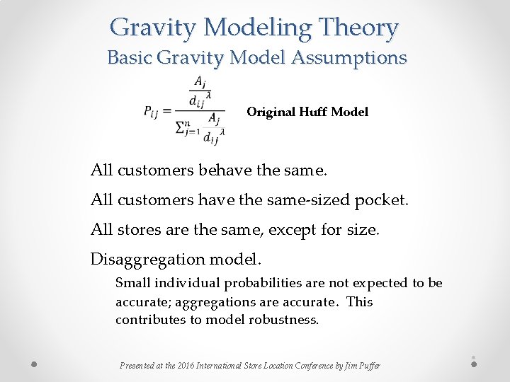
Gravity Modeling Theory Basic Gravity Model Assumptions Original Huff Model All customers behave the same. All customers have the same-sized pocket. All stores are the same, except for size. Disaggregation model. Small individual probabilities are not expected to be accurate; aggregations are accurate. This contributes to model robustness. Presented at the 2016 International Store Location Conference by Jim Puffer ●

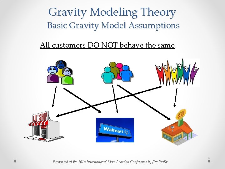
Gravity Modeling Theory Basic Gravity Model Assumptions All customers DO NOT behave the same. Presented at the 2016 International Store Location Conference by Jim Puffer ●

Gravity Modeling Theory Basic Gravity Model Assumptions All customers DO NOT behave the same. How we “fix” that violation: We create consumer profiles. We recognize store types. We research preferences. e. g. FIT Each product implements differently. Presented at the 2016 International Store Location Conference by Jim Puffer ●

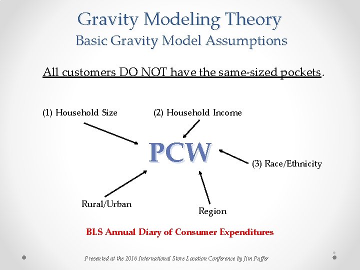
Gravity Modeling Theory Basic Gravity Model Assumptions All customers DO NOT have the same-sized pockets. (1) Household Size (2) Household Income PCW Rural/Urban (3) Race/Ethnicity Region BLS Annual Diary of Consumer Expenditures Presented at the 2016 International Store Location Conference by Jim Puffer ●

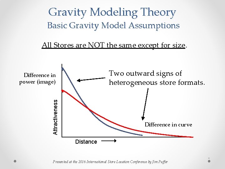
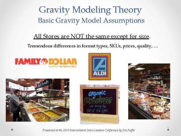
Gravity Modeling Theory Basic Gravity Model Assumptions All Stores are NOT the same except for size. Two outward signs of heterogeneous store formats. Attractiveness Difference in power (image) Difference in curve Distance Presented at the 2016 International Store Location Conference by Jim Puffer ●

Gravity Modeling Theory Basic Gravity Model Assumptions All Stores are NOT the same except for size. Tremendous differences in format types, SKUs, prices, quality, … Presented at the 2016 International Store Location Conference by Jim Puffer ●

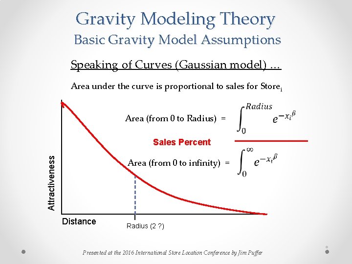
Gravity Modeling Theory Basic Gravity Model Assumptions Speaking of Curves (Gaussian model) … Area under the curve is proportional to sales for Storei Area (from 0 to Radius) = Attractiveness Sales Percent Area (from 0 to infinity) = Distance Radius (2 ? ) Presented at the 2016 International Store Location Conference by Jim Puffer ●

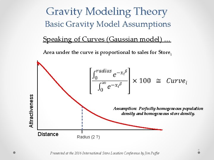
Gravity Modeling Theory Basic Gravity Model Assumptions Speaking of Curves (Gaussian model) … Attractiveness Area under the curve is proportional to sales for Storei Assumption: Perfectly homogeneous population density and homogeneous store density. Distance Radius (2 ? ) Presented at the 2016 International Store Location Conference by Jim Puffer ●

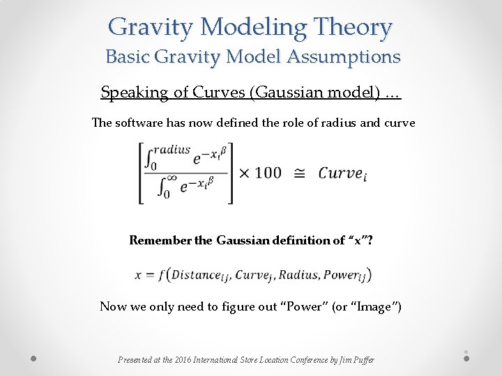
Gravity Modeling Theory Basic Gravity Model Assumptions Speaking of Curves (Gaussian model) … The software has now defined the role of radius and curve Remember the Gaussian definition of “x”? Now we only need to figure out “Power” (or “Image”) Presented at the 2016 International Store Location Conference by Jim Puffer ●

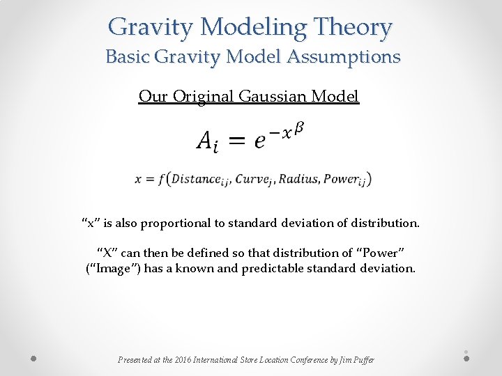
Gravity Modeling Theory Basic Gravity Model Assumptions Our Original Gaussian Model “x” is also proportional to standard deviation of distribution. “X” can then be defined so that distribution of “Power” (“Image”) has a known and predictable standard deviation. Presented at the 2016 International Store Location Conference by Jim Puffer ●

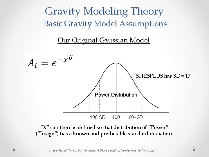
Gravity Modeling Theory Basic Gravity Model Assumptions Our Original Gaussian Model SITESPLUS has SD = 17 Power Distribution 100 -SD 100+SD “X” can then be defined so that distribution of “Power” (“Image”) has a known and predictable standard deviation. Presented at the 2016 International Store Location Conference by Jim Puffer ●

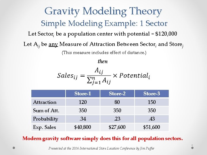
Gravity Modeling Theory Simple Modeling Example: 1 Sector Let Sectori be a population center with potential = $120, 000 Let Aij be any Measure of Attraction Between Sectori and Storej (This measure includes effect of distance. ) then Store-1 Store-2 Store-3 Attraction 120 80 150 Sum of Att. 350 350 Probability . 34 . 23 . 43 Exp. Sales $40, 800 $27, 600 $51, 600 Modern gravity software simply does this for all population sectors. Presented at the 2016 International Store Location Conference by Jim Puffer ●