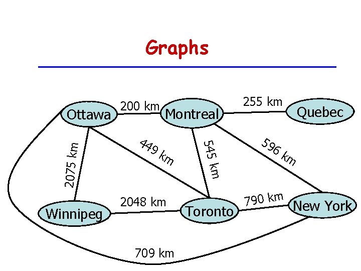
Graphs Winnipeg 44 Montreal 9 k m 2048

Graphs Winnipeg 44 Montreal 9 k m 2048 km 709 km m 545 k 2075 km Ottawa 200 km 255 km 59 Quebec 6 k m 790 km New York Toronto

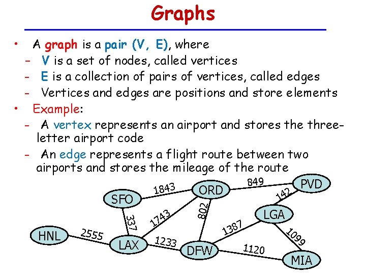
Graphs • HNL 2555 LAX 1 1233 802 337 A graph is a pair (V, E), where – V is a set of nodes, called vertices – E is a collection of pairs of vertices, called edges – Vertices and edges are positions and store elements • Example: – A vertex represents an airport and stores the threeletter airport code – An edge represents a flight route between two airports and stores the mileage of the route 849 PVD 3 ORD 184 2 14 SFO 3 LGA 74 7 138 DFW 1120 10 99 MIA

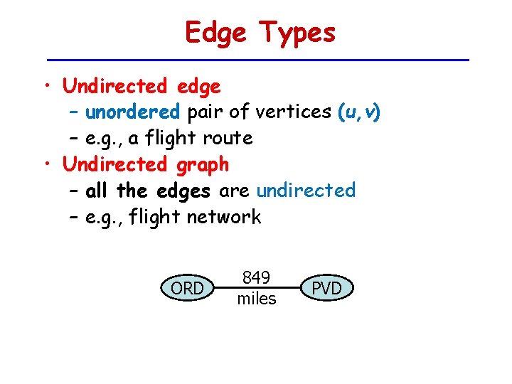
Edge Types • Undirected edge – unordered pair of vertices (u, v) – e. g. , a flight route • Undirected graph – all the edges are undirected – e. g. , flight network ORD 849 miles PVD

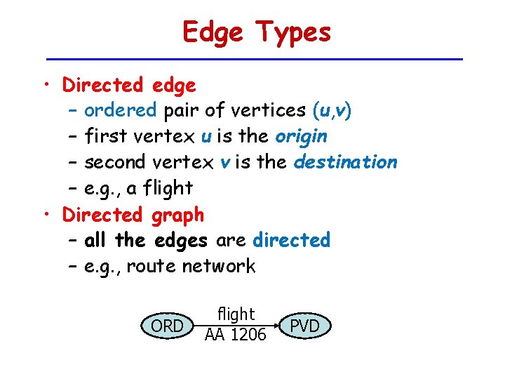
Edge Types • Directed edge – ordered pair of vertices (u, v) – first vertex u is the origin – second vertex v is the destination – e. g. , a flight • Directed graph – all the edges are directed – e. g. , route network ORD flight AA 1206 PVD

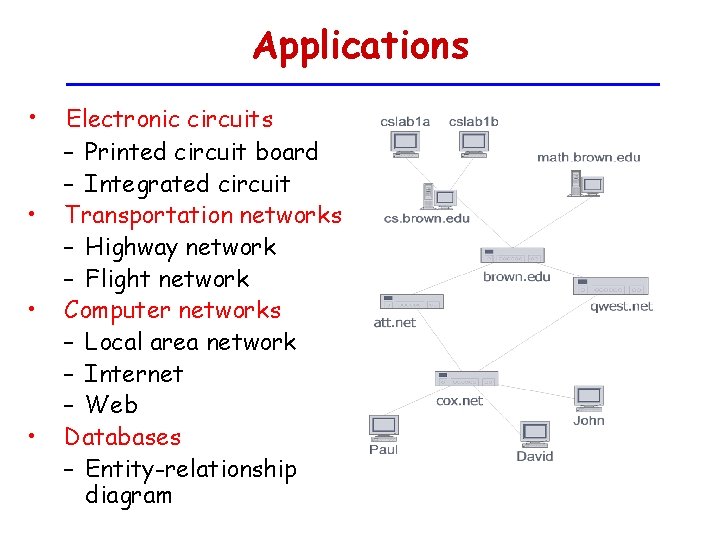
Applications • Electronic circuits • • • – Printed circuit board – Integrated circuit Transportation networks – Highway network – Flight network Computer networks – Local area network – Internet – Web Databases – Entity-relationship diagram

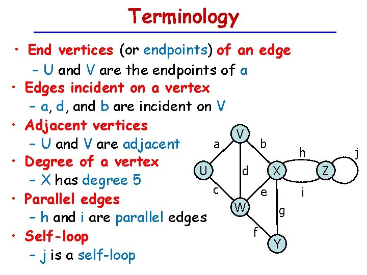
Terminology • End vertices (or endpoints) of an edge – U and V are the endpoints of a • Edges incident on a vertex – a, d, and b are incident on V • Adjacent vertices V b a – U and V are adjacent h • Degree of a vertex U d X – X has degree 5 c e i • Parallel edges W g – h and i are parallel edges f • Self-loop Y – j is a self-loop j Z

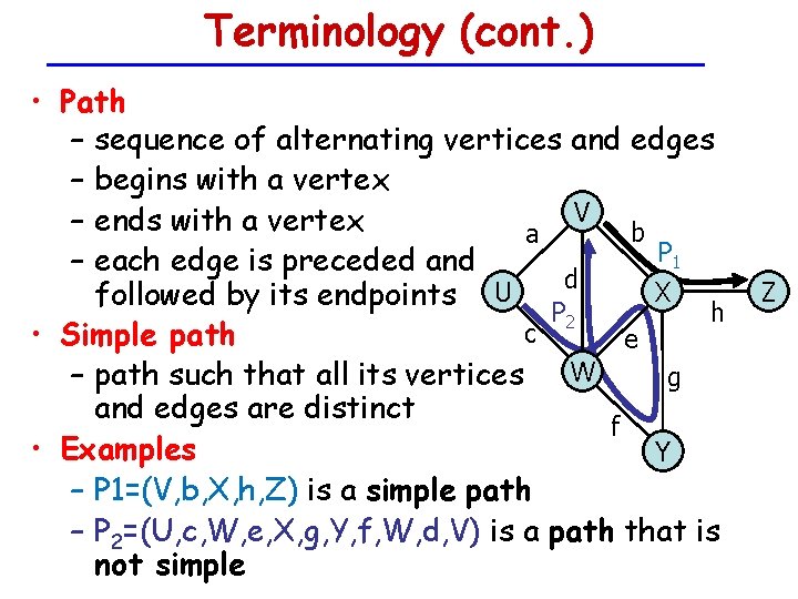
Terminology (cont. ) • Path – sequence of alternating vertices and edges – begins with a vertex V – ends with a vertex b a P 1 – each edge is preceded and d U X followed by its endpoints P 2 h c • Simple path e – path such that all its vertices W g and edges are distinct f • Examples Y – P 1=(V, b, X, h, Z) is a simple path – P 2=(U, c, W, e, X, g, Y, f, W, d, V) is a path that is not simple Z

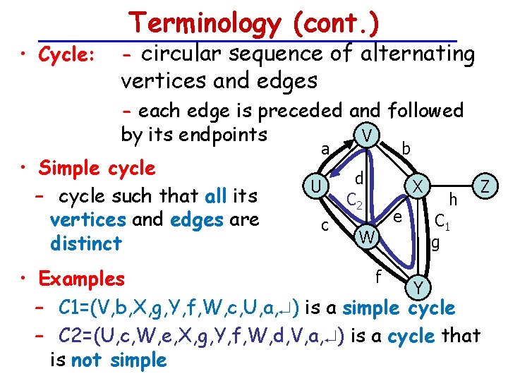
• Cycle: Terminology (cont. ) - circular sequence of alternating vertices and edges - each edge is preceded and followed by its endpoints V • Simple cycle – cycle such that all its vertices and edges are distinct a U c b d C 2 W X e h Z C 1 g f • Examples Y – C 1=(V, b, X, g, Y, f, W, c, U, a, ) is a simple cycle – C 2=(U, c, W, e, X, g, Y, f, W, d, V, a, ) is a cycle that is not simple

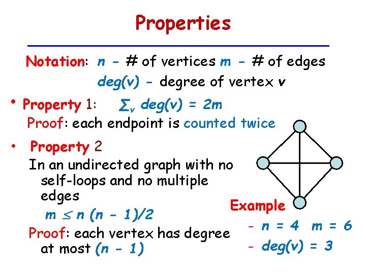
Properties Notation: n - # of vertices m - # of edges deg(v) - degree of vertex v • Property 1: ∑v deg(v) = 2 m Proof: each endpoint is counted twice • Property 2 In an undirected graph with no self-loops and no multiple edges Example m n (n - 1)/2 – n = 4 m = 6 Proof: each vertex has degree – deg(v) = 3 at most (n - 1)

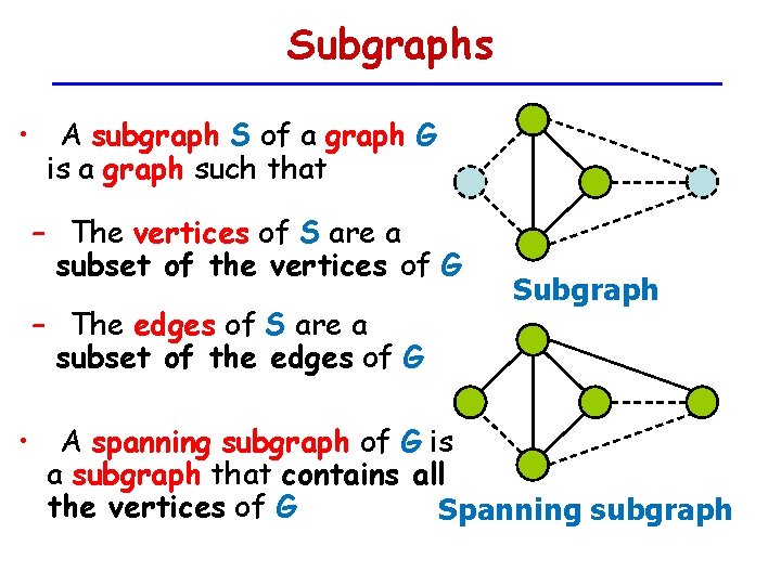
Subgraphs • A subgraph S of a graph G is a graph such that – The vertices of S are a subset of the vertices of G – The edges of S are a subset of the edges of G Subgraph • A spanning subgraph of G is a subgraph that contains all the vertices of G Spanning subgraph

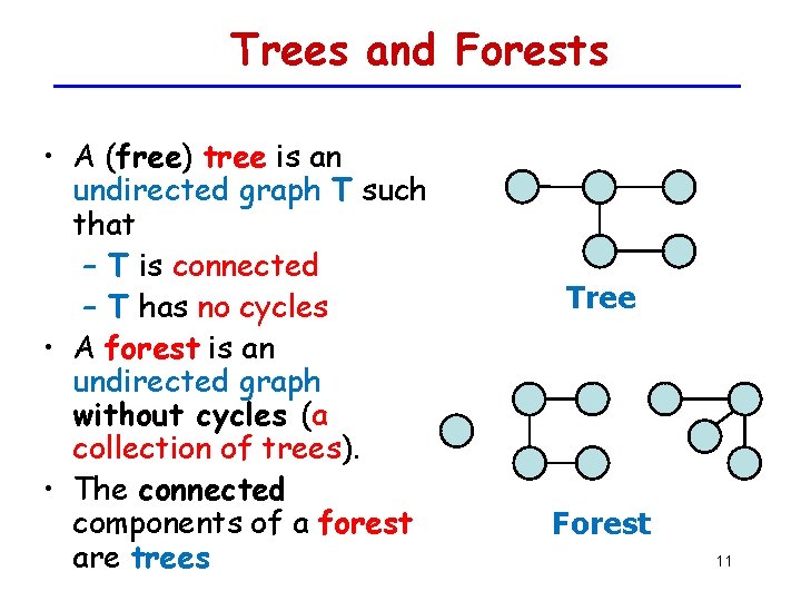
Trees and Forests • A (free) tree is an undirected graph T such that – T is connected – T has no cycles • A forest is an undirected graph without cycles (a collection of trees). • The connected components of a forest are trees Tree Forest 11

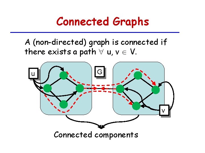
Connected Graphs A (non-directed) graph is connected if there exists a path u, v V. u G v Connected components

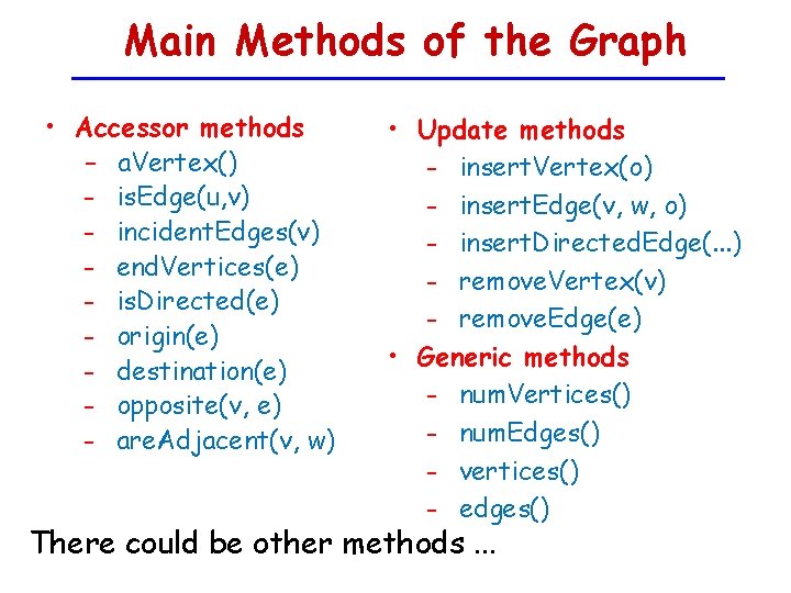
Main Methods of the Graph • Accessor methods – a. Vertex() – is. Edge(u, v) – incident. Edges(v) – end. Vertices(e) – is. Directed(e) – origin(e) – destination(e) – opposite(v, e) – are. Adjacent(v, w) • Update methods – insert. Vertex(o) – insert. Edge(v, w, o) – insert. Directed. Edge(. . . ) – remove. Vertex(v) – remove. Edge(e) • Generic methods – num. Vertices() – num. Edges() – vertices() – edges() There could be other methods. . .

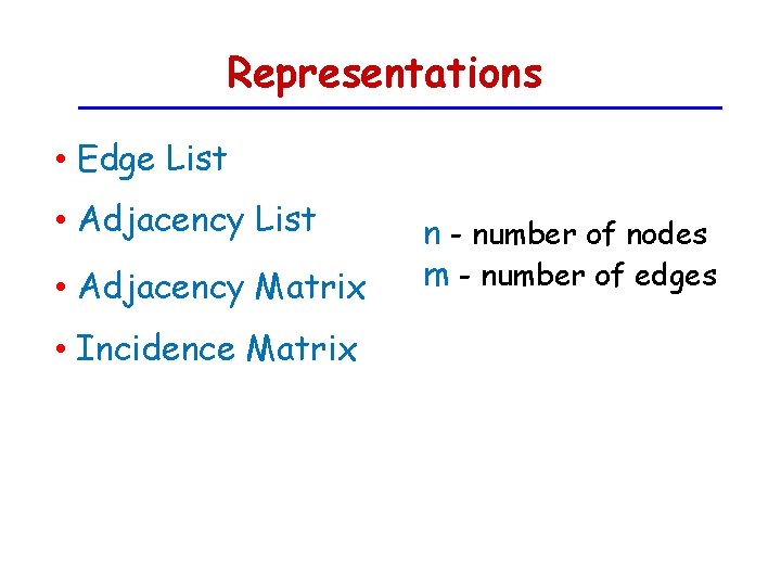
Representations • Edge List • Adjacency Matrix • Incidence Matrix n - number of nodes m - number of edges

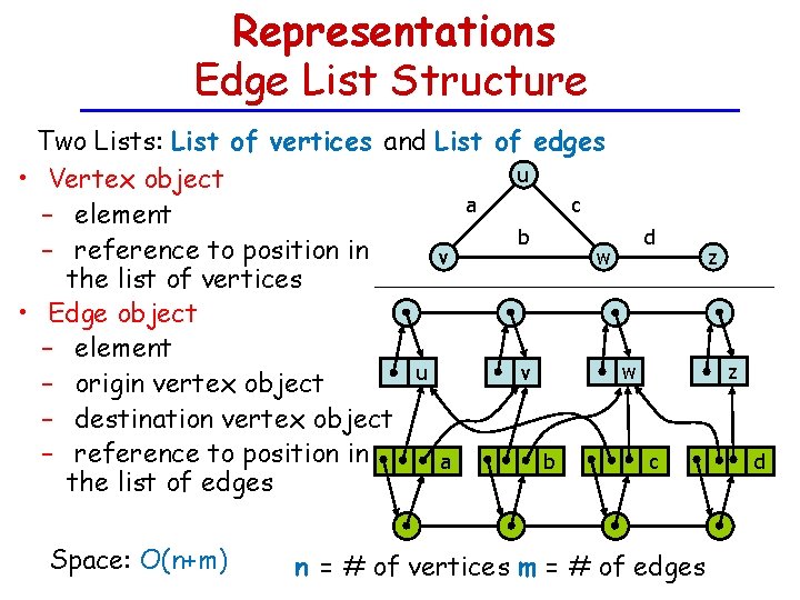
Representations Edge List Structure Two Lists: List of vertices and List of edges u • Vertex object a c – element b – reference to position in v w the list of vertices • Edge object – element u v – origin vertex object – destination vertex object – reference to position in a b the list of edges Space: O(n+m) d z z w c n = # of vertices m = # of edges d

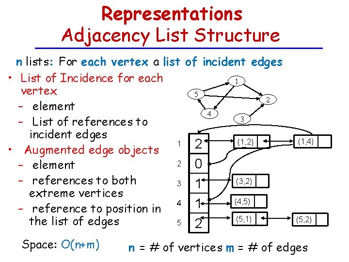
Representations Adjacency List Structure n lists: For each vertex a list of incident edges • List of Incidence for each 1 vertex 5 2 – element 4 3 – List of references to incident edges (1, 2) 1 2 • Augmented edge objects 2 0 – element (3, 2) – references to both 3 1 extreme vertices (4, 5) 4 1 – reference to position in (5, 1) the list of edges 5 2 Space: O(n+m) (1, 4) (5, 2) n = # of vertices m = # of edges

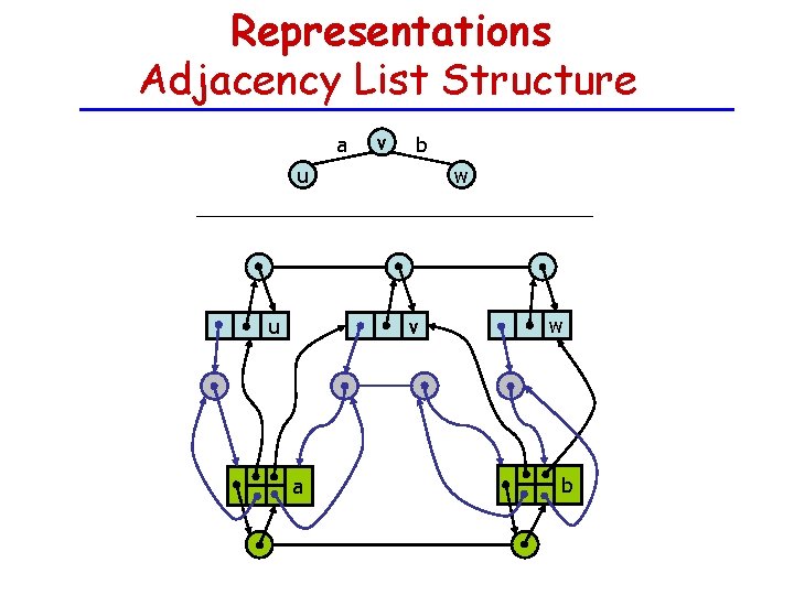
Representations Adjacency List Structure a v b u u w v a w b

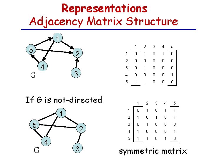
Representations Adjacency Matrix Structure 1 5 2 G 4 3 1 2 3 4 5 1 0 1 0 2 0 0 0 3 0 1 0 0 0 4 0 0 1 5 1 1 0 0 0 If G is not-directed 1 5 G 2 4 3 1 2 3 4 5 1 0 1 1 2 1 0 1 3 0 1 0 0 0 4 1 0 0 0 1 5 1 1 0 symmetric matrix

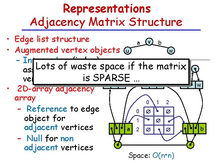
Representations Adjacency Matrix Structure • Edge list structure a v b w • Augmented vertex objects u – Integer key (index) Lots ofwith waste space if the matrix associated is SPARSE … vertex 2 0 u 1 v • 2 D-array adjacency array 0 1 2 – Reference to edge 0 object for 1 adjacent vertices a 2 – Null for non adjacent vertices Space: O(n*n) w b

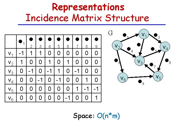
Representations Incidence Matrix Structure 1 2 3 4 5 v 1 -1 1 1 0 0 v 2 1 0 0 1 0 v 3 0 -1 1 v 4 0 0 -1 v 5 0 0 0 v 6 0 0 0 6 7 8 9 0 1 0 0 0 -1 0 1 0 0 1 -1 0 0 0 -1 1 G 1 v 2 4 6 Space: O(n*m) v 1 2 v 3 v 6 9 3 5 v 4 8 7 v 5

Is (vi, vj) an edge? j Adjacency Matrix: i Adjacency List: [ ] O(1) i j … Min{O(deg(i)), O(deg(j))} Edge List: l 1 l 2 l 3 l 4 l 5 l 6 l 7 l 8 l 9 O(m) v 1 v 2 v 3 v 4 v 5 v 6

Which nodes are adjacent to vi? Adjacency Matrix: i Adjacency List: [ ] O(n) i O(deg(i)) Edge List: l 1 l 2 l 3 l 4 l 5 l 6 l 7 l 8 l 9 O(m) v 1 v 2 v 3 v 4 v 5 v 6

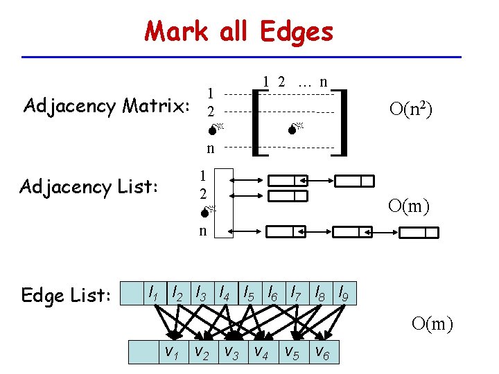
Mark all Edges Adjacency Matrix: Adjacency List: Edge List: 1 2 n 1 2 … n [ ] O(n 2) 1 2 n O(m) l 1 l 2 l 3 l 4 l 5 l 6 l 7 l 8 l 9 O(m) v 1 v 2 v 3 v 4 v 5 v 6

Add an Edge (vi, vj) j Adjacency Matrix: i Adjacency List: [ ] 1 O(1) i O(1) Edge List: l 1 l 2 l 3 l 4 l 5 l 6 l 7 l 8 l 9 O(1) v 1 v 2 v 3 v 4 v 5 v 6

Remove an Edge (vi, vj) j Adjacency Matrix: i Adjacency List: [ ] 0 i O(1) j O(1) Edge List: l 1 l 2 l 3 l 4 l 5 l 6 l 7 l 8 l 9 O(1) v 1 v 2 v 3 v 4 v 5 v 6

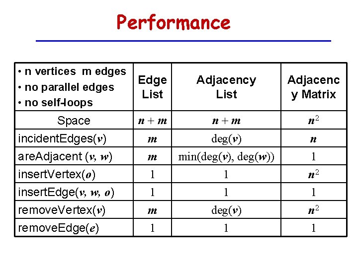
Performance • n vertices m edges • no parallel edges • no self-loops Edge List Adjacency List Adjacenc y Matrix Space n+m n 2 incident. Edges(v) are. Adjacent (v, w) insert. Vertex(o) m m 1 deg(v) min(deg(v), deg(w)) 1 n 2 insert. Edge(v, w, o) 1 1 1 remove. Vertex(v) remove. Edge(e) m 1 deg(v) 1 n 2 1

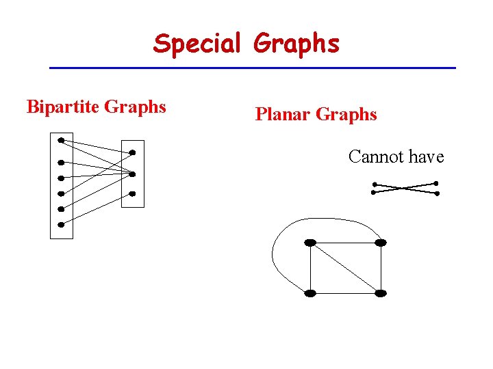
Special Graphs Bipartite Graphs Planar Graphs Cannot have

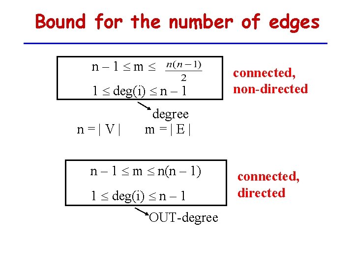
Bound for the number of edges n– 1 m 1 deg(i) n – 1 n=|V| connected, non-directed degree m=|E| n – 1 m n(n – 1) 1 deg(i) n – 1 OUT-degree connected, directed

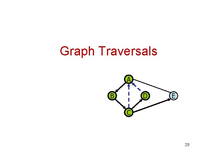
Graph Traversals A B D E C 29

Graph Traversals A traversal of a graph G: – – – Visits all the vertices and edges of G Determines whether G is connected Computes the connected components of G Computes a spanning forest of G Build a spanning tree in a connected graph 30

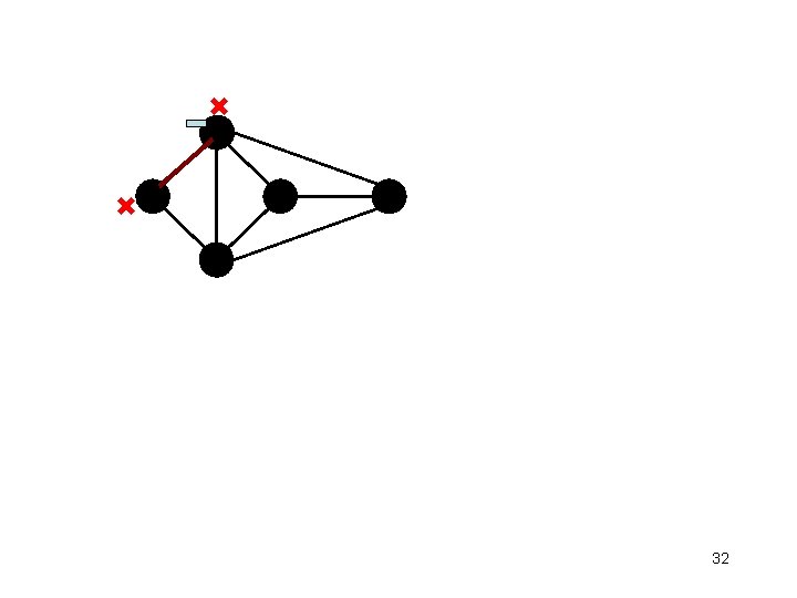
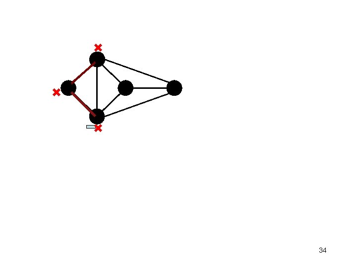
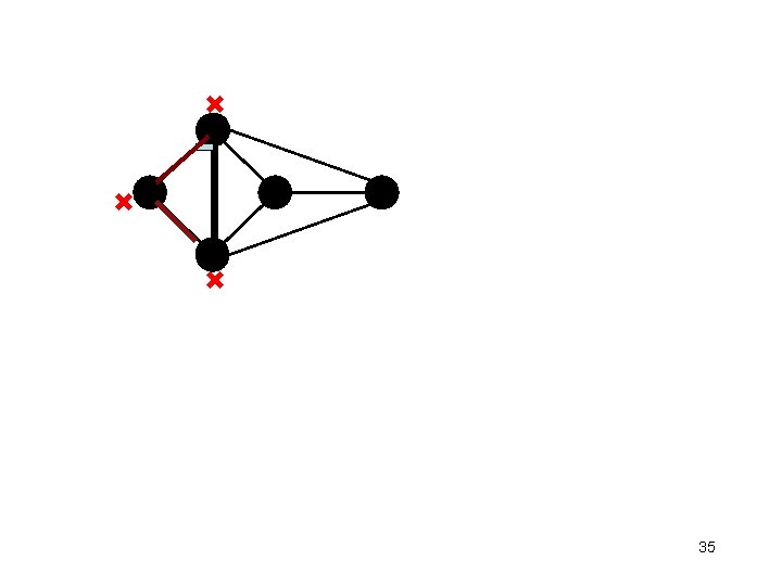
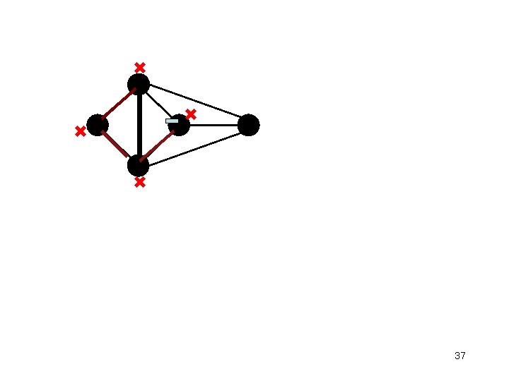
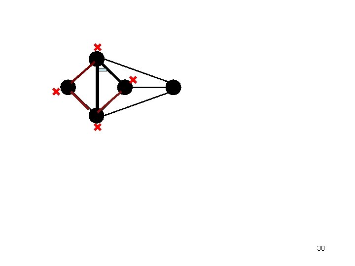
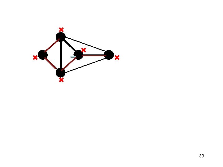
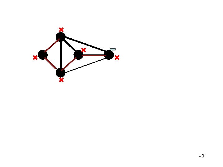
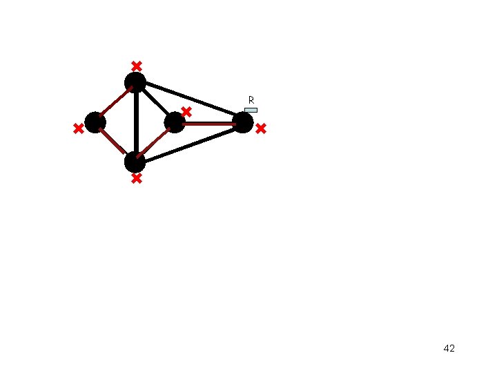
Depth-First Search (DFS) is a graph traversal technique that: • on a graph with n vertices and m edges takes O(n + m ) time (which is O(m) ) • can be further extended to solve other graph problems – Find and report a path between two given vertices Find a cycle in the graph, if there is one The idea: Starting at an arbitrary vertex, follow along a simple path until you get to a vertex which has no unvisited adjacent vertices. Then start tracing back up the path, one vertex at a time, to find a vertex with unvisited adjacent vertices.

32

33

34

35

36

37

38

39

40

41

R 42

R 43

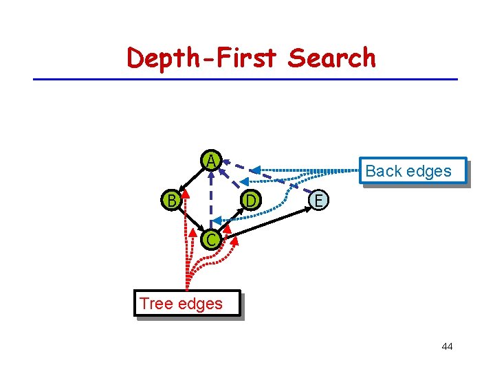
Depth-First Search A B Back edges D E C Tree edges 44

DFS Algorithm – With a Stack • When we arrive to a node for the first time: − We push all its incident edges to the stack − We add the edge from where we came to the tree. • To move to a new node we remove the first edge in the stack and move through it.

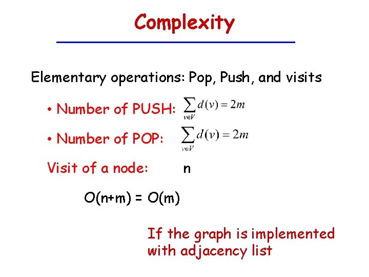
Complexity Elementary operations: Pop, Push, and visits • Number of PUSH: • Number of POP: Visit of a node: n O(n+m) = O(m) If the graph is implemented with adjacency list

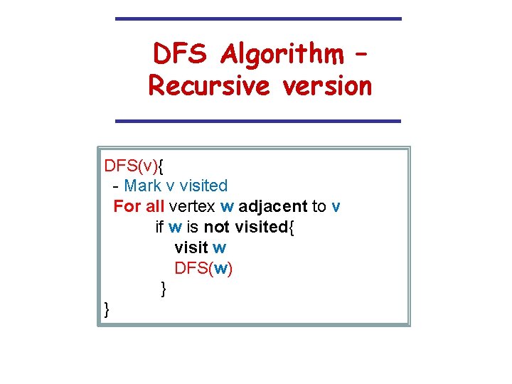
DFS Algorithm – Recursive version DFS(v){ - Mark v visited For all vertex w adjacent to v if w is not visited{ visit w DFS(w) } }

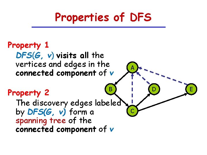
Properties of DFS Property 1 DFS(G, v) visits all the vertices and edges in the connected component of v B Property 2 The discovery edges labeled by DFS(G, v) form a spanning tree of the connected component of v A D C E

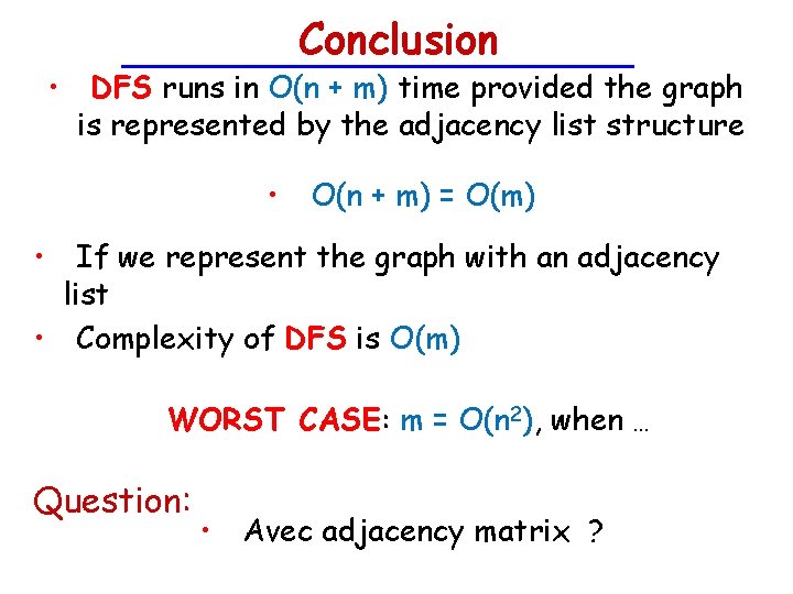
Conclusion • DFS runs in O(n + m) time provided the graph is represented by the adjacency list structure • O(n + m) = O(m) • If we represent the graph with an adjacency list • Complexity of DFS is O(m) WORST CASE: m = O(n 2), when … Question: • Avec adjacency matrix ?

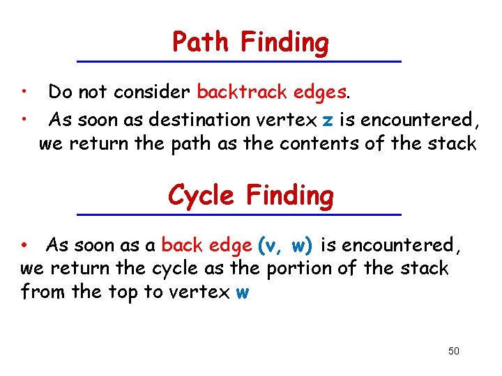
Path Finding • Do not consider backtrack edges. • As soon as destination vertex z is encountered, we return the path as the contents of the stack Cycle Finding • As soon as a back edge (v, w) is encountered, we return the cycle as the portion of the stack from the top to vertex w 50

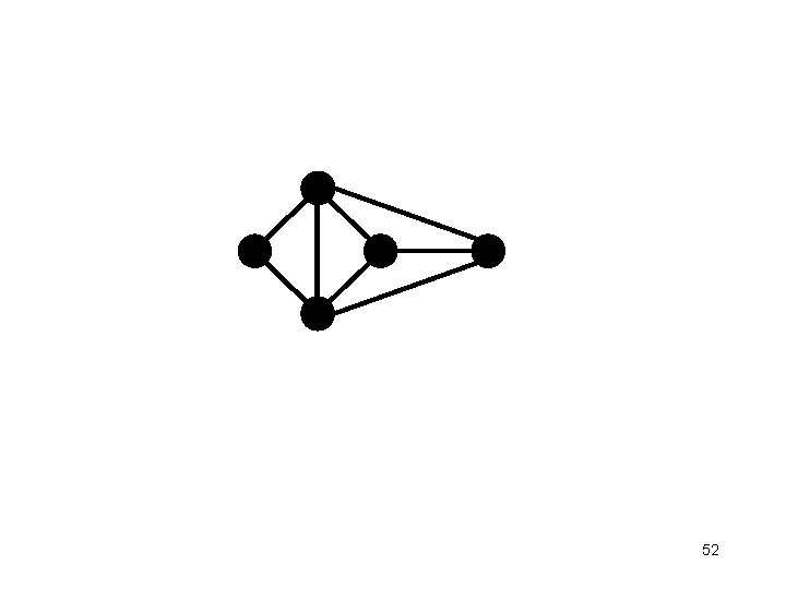
Breadth-First Search (BFS) is a graph traversal technique that: • on a graph with n vertices and m edges takes O(n + m ) time (which is O(m) ) • can be further extended to solve other graph problems – Find and report a path with the minimum number of edges between two given vertices Find a simple cycle, if there is one The idea: Visit a vertex and then visit all unvisited vertices that are adjacent to it before visiting a vertex which is 2 nodes away from it.

52

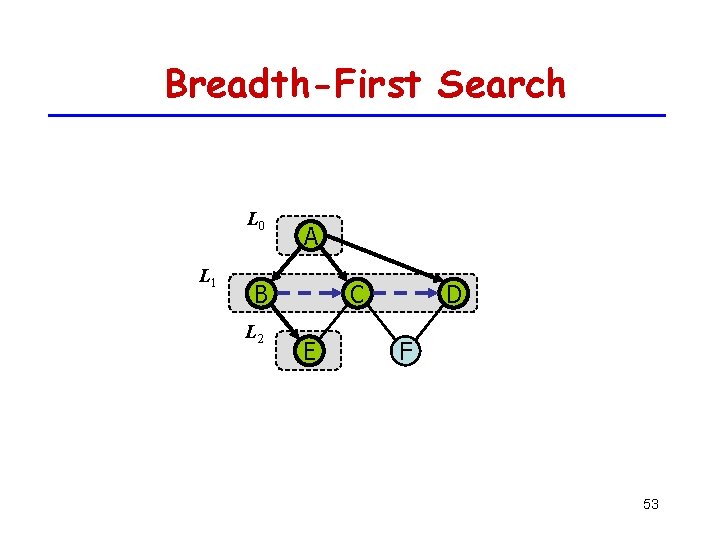
Breadth-First Search L 0 L 1 A B L 2 C E D F 53

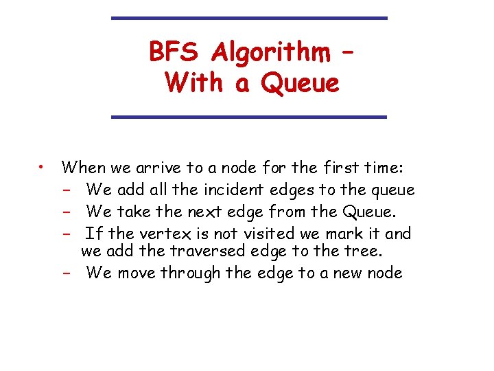
BFS Algorithm – With a Queue • When we arrive to a node for the first time: − We add all the incident edges to the queue − We take the next edge from the Queue. − If the vertex is not visited we mark it and we add the traversed edge to the tree. − We move through the edge to a new node

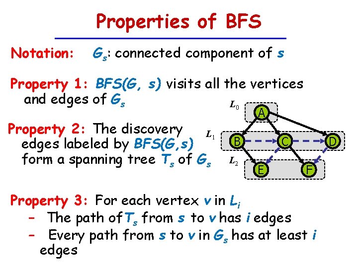
Properties of BFS Notation: Gs: connected component of s Property 1: BFS(G, s) visits all the vertices and edges of Gs L 0 Property 2: The discovery L 1 edges labeled by BFS(G, s) form a spanning tree Ts of Gs A B L 2 C E D F Property 3: For each vertex v in Li − The path of. Ts from s to v has i edges – Every path from s to v in Gs has at least i edges

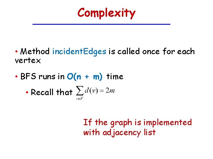
Complexity • Method incident. Edges is called once for each vertex • BFS runs in O(n + m) time • Recall that If the graph is implemented with adjacency list

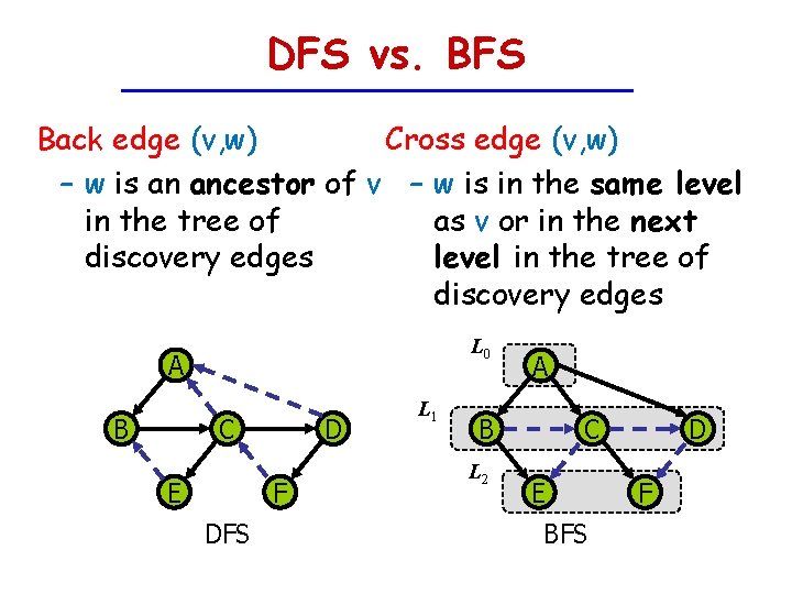
DFS vs. BFS Back edge (v, w) Cross edge (v, w) – w is an ancestor of v – w is in the same level in the tree of as v or in the next discovery edges level in the tree of discovery edges L 0 A B C E D F DFS L 1 A B L 2 C E BFS D F

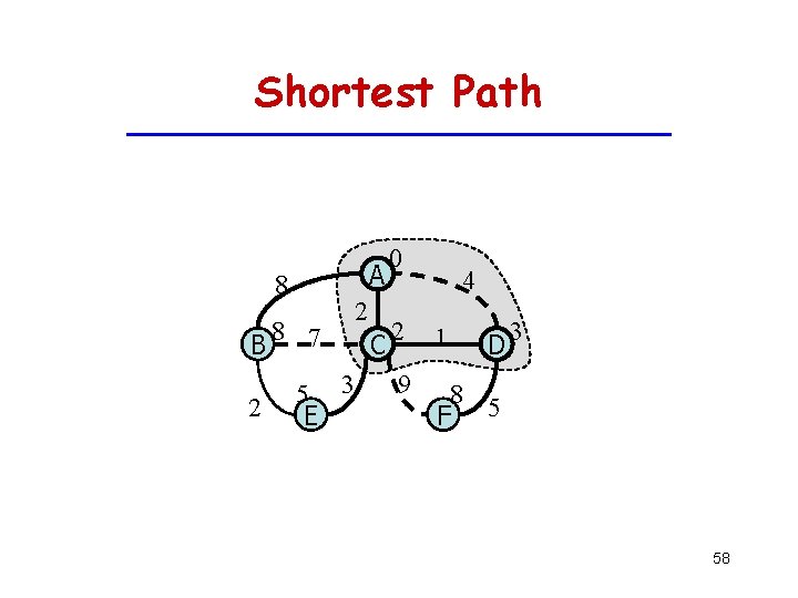
Shortest Path A 8 8 7 B 2 2 5 3 E C 0 4 2 1 9 8 F 5 D 3 58

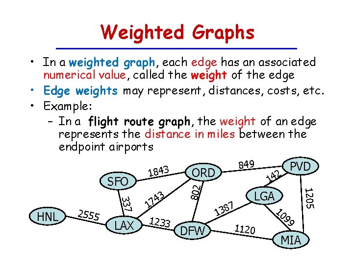
Weighted Graphs • In a weighted graph, each edge has an associated numerical value, called the weight of the edge • Edge weights may represent, distances, costs, etc. • Example: – In a flight route graph, the weight of an edge represents the distance in miles between the endpoint airports LAX 1233 ORD 1 802 337 HNL 2555 3 4 17 849 7 138 DFW 42 PVD 1205 SFO 1843 LGA 1120 10 99 MIA

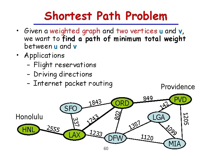
Shortest Path Problem • Given a weighted graph and two vertices u and v, we want to find a path of minimum total weight between u and v • Applications – Flight reservations – Driving directions – Internet packet routing Providence HNL 2555 43 7 1 LAX 1233 ORD 802 337 Honolulu 849 DFW 60 7 8 3 1 2 14 PVD 1205 SFO 1843 LGA 1120 10 99 MIA

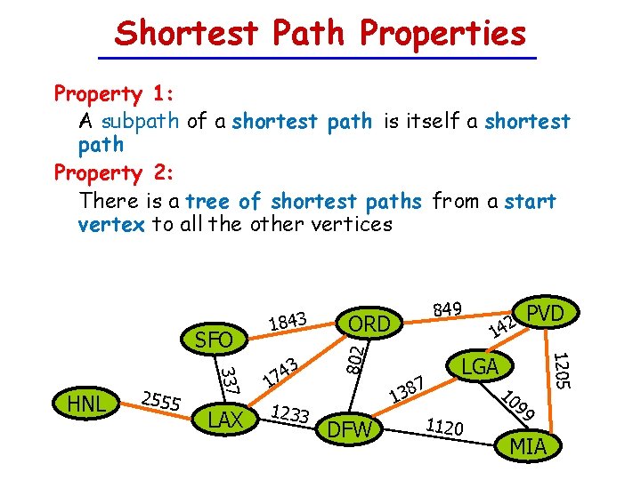
Shortest Path Properties Property 1: A subpath of a shortest path is itself a shortest path Property 2: There is a tree of shortest paths from a start vertex to all the other vertices LAX 1233 ORD 1 802 337 HNL 2555 3 4 17 849 7 138 DFW 42 PVD 1205 SFO 1843 LGA 1120 10 99 MIA

Dijkstra’s Algorithm • The distance of a vertex v from a vertex s is the length of a shortest path between s and v • Dijkstra’s algorithm computes the distances of all the vertices from a given start vertex s • Assumptions: – the graph is connected – the edges are undirected – the edge weights are nonnegative

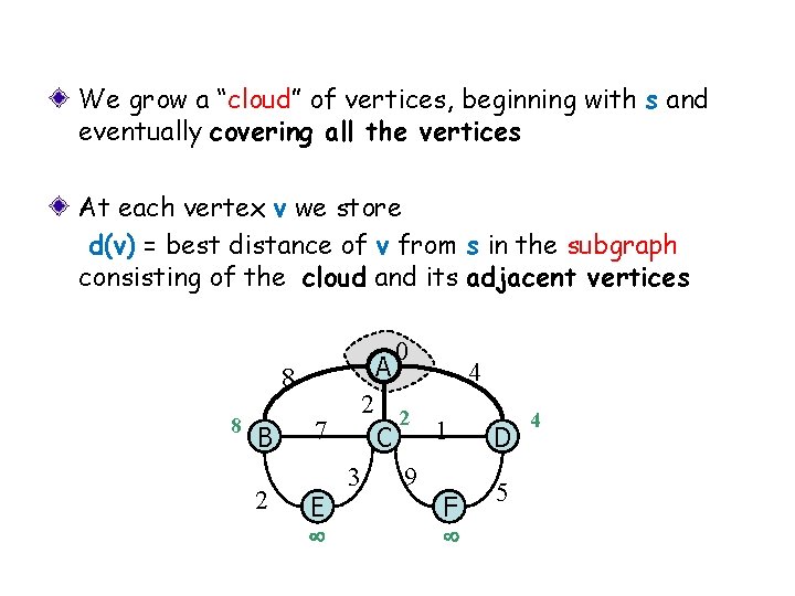
We grow a “cloud” of vertices, beginning with s and eventually covering all the vertices At each vertex v we store d(v) = best distance of v from s in the subgraph consisting of the cloud and its adjacent vertices 8 8 B 2 A 0 4 2 2 7 1 C 3 9 E F D 5 4

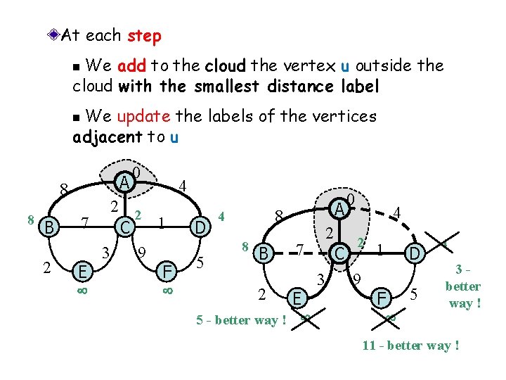
At each step We add to the cloud the vertex u outside the cloud with the smallest distance label n We update the labels of the vertices adjacent to u n 8 8 B 2 A 0 4 2 2 7 1 C 3 9 E F D 5 A 8 4 8 B 2 2 7 E 5 - better way ! C 3 0 4 2 9 1 D F 5 4 3 better way ! 11 - better way !

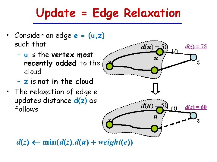
Update = Edge Relaxation • Consider an edge e = (u, z) such that – u is the vertex most recently added to the s cloud – z is not in the cloud • The relaxation of edge e updates distance d(z) as follows s d(z) min(d(z), d(u) + weight(e)) d(u) = 50 u 10 d(u) = 50 10 u d(z) = 75 z d(z) = 60 z

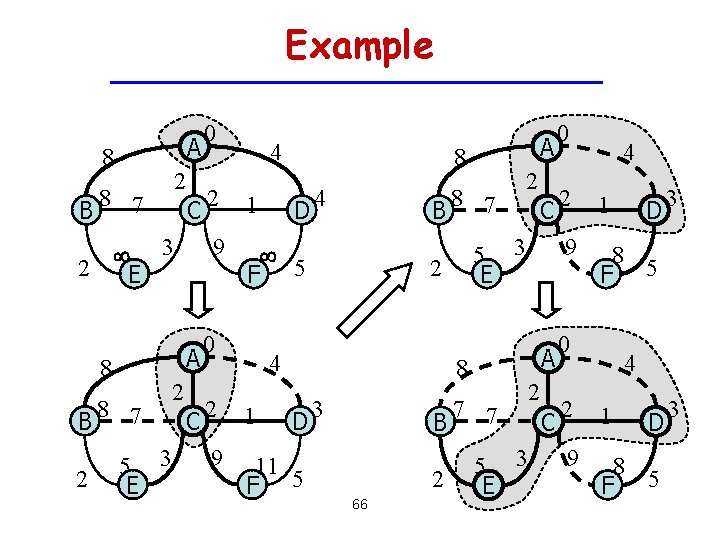
Example A 8 B 2 8 7 C 3 2 E A 8 B 2 8 7 2 5 3 E C 0 4 8 2 1 9 F 5 0 A D 4 B 8 7 C 5 3 E 2 4 2 A 8 2 1 9 11 F 5 D 3 B 2 66 7 7 2 5 3 E C 0 4 2 1 9 8 F 5 0 D 3 4 2 1 9 8 F 5 D 3

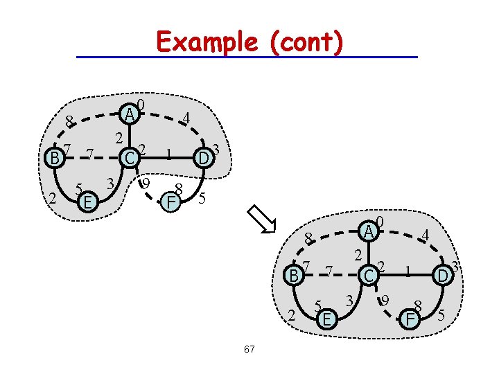
Example (cont) A 8 2 7 7 B 2 5 E C 3 0 4 2 1 9 8 F 5 D 3 A 8 B 2 67 2 7 7 5 E C 3 0 4 2 1 9 8 F 5 D 3

Dijkstra’s Algorithm we use a priority queue Q to store the vertices not in the cloud, where D[v] is the key of a vertex v in Q 68

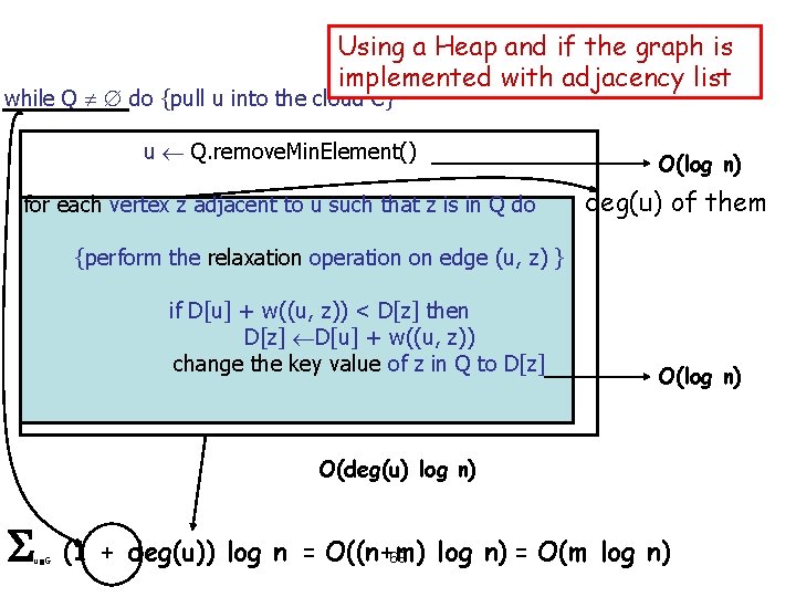
Using a Heap and if the graph is implemented with adjacency list while Q do {pull u into the cloud C} u Q. remove. Min. Element() for each vertex z adjacent to u such that z is in Q do O(log n) deg(u) of them {perform the relaxation operation on edge (u, z) } if D[u] + w((u, z)) < D[z] then D[z] D[u] + w((u, z)) change the key value of z in Q to D[z] O(log n) O(deg(u) log n) u G (1 + deg(u)) log n = O((n+m) log n) = O(m log n) 69

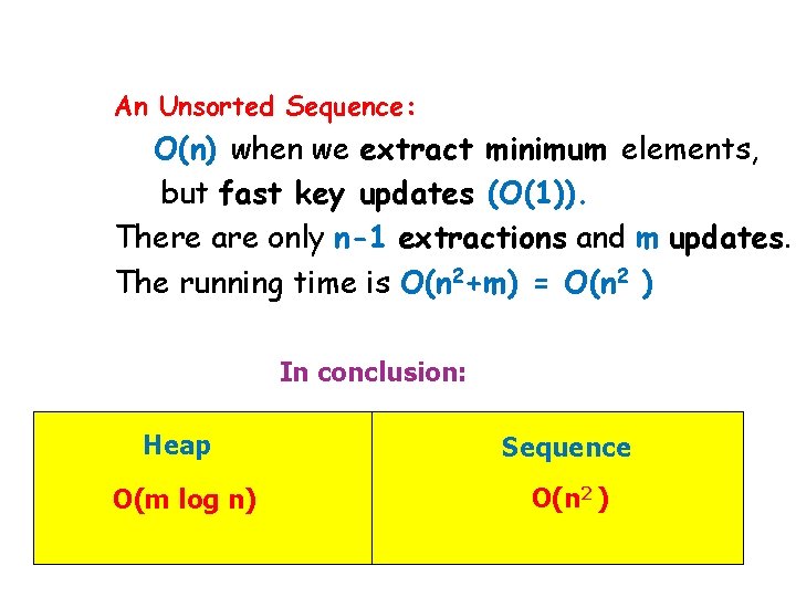
An Unsorted Sequence: O(n) when we extract minimum elements, but fast key updates (O(1)). There are only n-1 extractions and m updates. The running time is O(n 2+m) = O(n 2 ) In conclusion: Heap Sequence O(m log n) O(n 2 ) 70

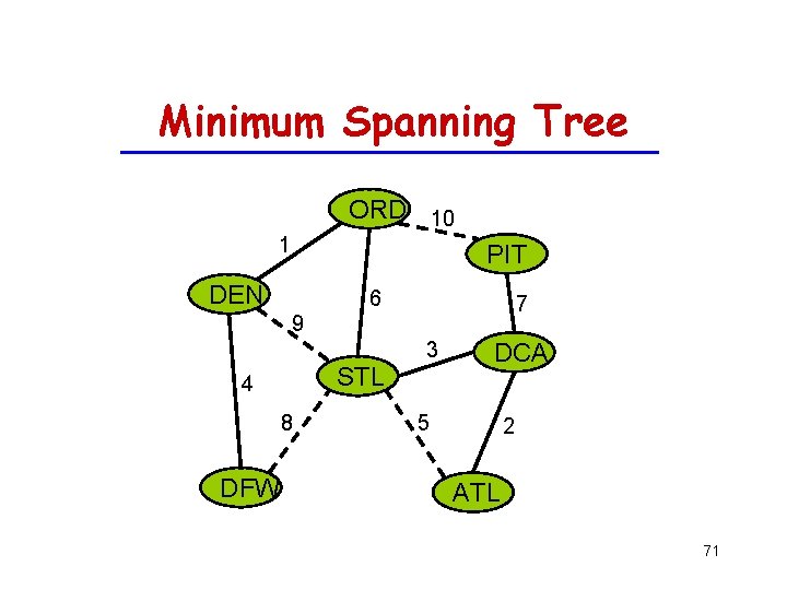
Minimum Spanning Tree ORD 10 1 PIT DEN 6 7 9 3 STL 4 8 DFW DCA 5 2 ATL 71

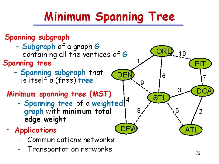
Minimum Spanning Tree Spanning subgraph – Subgraph of a graph G containing all the vertices of G 1 Spanning tree – Spanning subgraph that DEN is itself a (free) tree 9 Minimum spanning tree (MST) 4 – Spanning tree of a weighted 8 graph with minimum total edge weight DFW • Applications – Communications networks – Transportation networks ORD 10 PIT 6 7 3 STL DCA 5 2 ATL 72

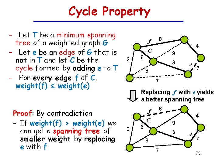
Cycle Property – Let T be a minimum spanning tree of a weighted graph G – Let e be an edge of G that is not in T and let C be the cycle formed by adding e to T – For every edge f of C, weight(f) weight(e) Proof: By contradiction – If weight(f) > weight(e) we can get a spanning tree of smaller weight by replacing e with f f 8 4 C 2 9 6 3 e 8 7 7 Replacing f with e yields a better spanning tree f 8 4 C 2 9 6 3 8 7 e 7 73

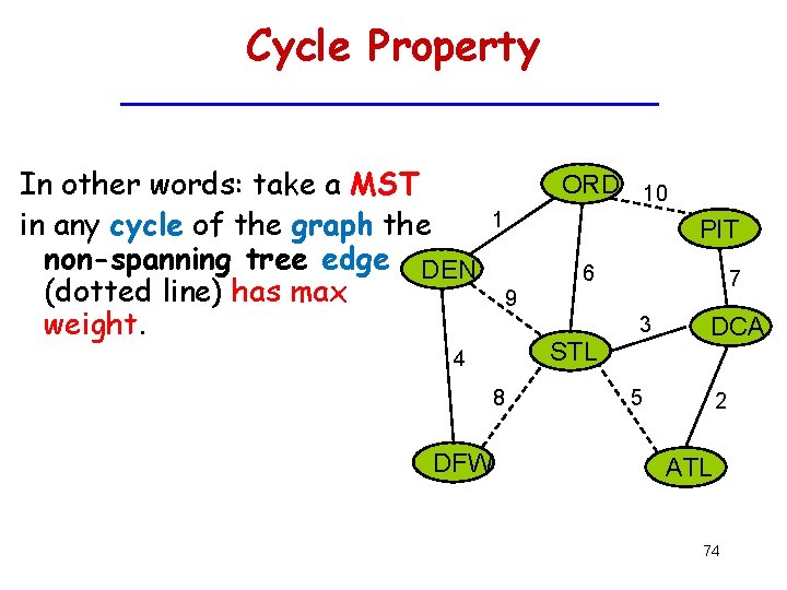
Cycle Property In other words: take a MST in any cycle of the graph the non-spanning tree edge DEN (dotted line) has max weight. ORD 10 1 PIT 6 9 3 STL 4 8 DFW 7 DCA 5 2 ATL 74

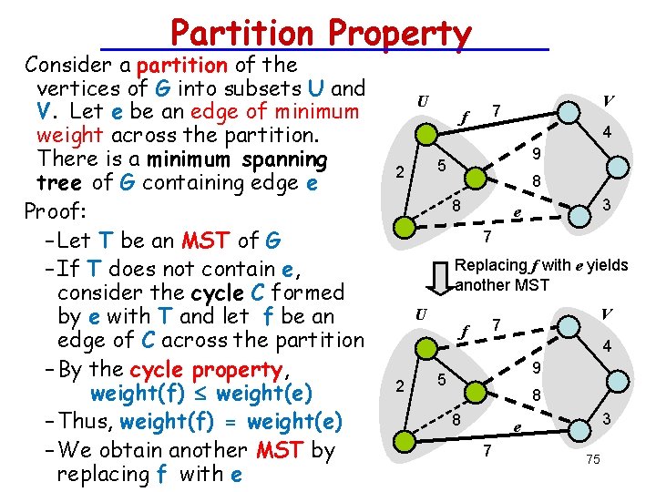
Partition Property Consider a partition of the vertices of G into subsets U and V. Let e be an edge of minimum weight across the partition. There is a minimum spanning tree of G containing edge e Proof: – Let T be an MST of G – If T does not contain e, consider the cycle C formed by e with T and let f be an edge of C across the partition – By the cycle property, weight(f) weight(e) – Thus, weight(f) = weight(e) – We obtain another MST by replacing f with e U f V 7 4 9 5 2 8 8 3 e 7 Replacing f with e yields another MST U 2 f V 7 4 9 5 8 8 3 e 7 75

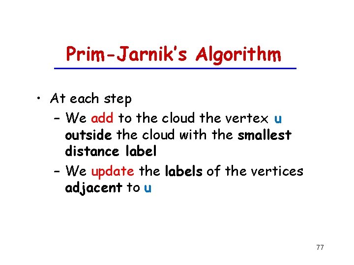
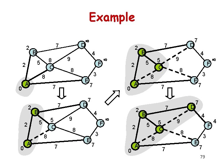
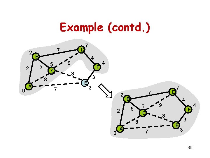
Prim-Jarnik’s Algorithm Prim-Jarnik’s algorithm for computing an MST is similar to Dijkstra’s algorithm We assume that the graph is connected We pick an arbitrary vertex s and we grow the MST as a cloud of vertices, starting from s We store with each vertex v a label d(v) representing the smallest weight of an edge connecting v to any vertex in the cloud (as opposed to the total sum of edge weights on a path from the start vertex to u). 76

Prim-Jarnik’s Algorithm • At each step – We add to the cloud the vertex u outside the cloud with the smallest distance label – We update the labels of the vertices adjacent to u 77

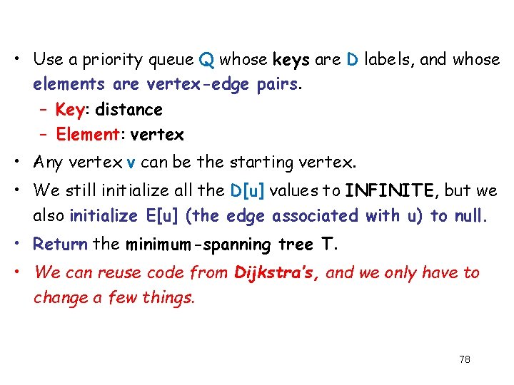
• Use a priority queue Q whose keys are D labels, and whose elements are vertex-edge pairs. – Key: distance – Element: vertex • Any vertex v can be the starting vertex. • We still initialize all the D[u] values to INFINITE, but we also initialize E[u] (the edge associated with u) to null. • Return the minimum-spanning tree T. • We can reuse code from Dijkstra’s, and we only have to change a few things. 78

Example 2 7 B F 8 8 0 A 2 2 E 5 C 0 F 8 0 A 2 E 7 4 9 F 8 2 3 7 0 7 7 B 5 C 5 8 A D 7 4 9 F 8 3 E 7 3 7 E 7 4 9 5 C 5 2 7 B 8 A D 7 3 7 5 2 4 9 8 C 5 2 D 7 79 4

Example (contd. ) 2 2 B 5 C 5 8 0 A D 7 7 4 9 F 8 3 E 7 4 3 2 2 B 5 C 5 8 0 A D 7 7 4 9 F 8 3 E 7 3 80 4

Analysis • Graph operations – Method incident. Edges is called once for each vertex • Label operations – We set/get the labels of vertex z O(deg(z)) times – Setting/getting a label takes O(1) time • Priority queue operations – Each vertex is inserted once into and removed once from the priority queue, where each insertion or removal takes O(log n) time – The key of a vertex w in the priority queue is modified at most deg(w) times, where each key change takes O(log n) time • Prim-Jarnik’s algorithm runs in O((n + m) log n) time provided the graph is represented by the adjacency list structure – Recall that Sv deg(v) = 2 m • The running time is O(m log n) since the graph is connected 81