Graphs and Finding your way in the wilderness

Graphs and Finding your way in the wilderness Chapter 14 in DS&PS Chapter 9 in DS&AA

General Problems • • What is the shortest path from A to B? What is the shortest path from A to all nodes? What is the shortest/cheapest path between any two nodes? . Search for Goal node, i. e. a node with specific properties, like a win in chess. • What is shortest tour? (visit all vertices) – no known polynomial algorithm in number of edges • What is longest path from A to B

Some Applications • Route Finding – metacrawler, on net, claims to find shortest path between two points • Game-Playing – great increase in chess/checkers end-game play occurred when recognized as graph search, not tree search • Critical Path Analysis – multiperson/task job schedule analysis – answers what are the key tasks that can’t slip • Travel arrangement – cheapest cost to meet constraints

Definitions • Graph: set of edges E and vertices V. • Edge is a pair of vertices (v, w) – edge may be directed or undirected – edge may have a cost – v and w are said to be adjacent • Digraph or directed graph: directed edges • Path: sequence of vertices v 1, …vn where each <vi, vi+1> is an edge. • Cycle: path where v 1=vn • Tour: cycle that contains every vertex • DAG: directed acyclic graph – graph with no cycles – Tree algorithms usually work with DAGs just fine

Adjacency Matrix Representation • Matrix A = new Boolean(|V|, |V|). – O(|V|^2) memory costs: acceptable only if dense • If <vi, vj> is an edge, set A[i][j] = true, else false • Special matrix multiple operator: – row[i] @ col[j] = row[i][1]&col[1][j] or row[i][2]&col[2][j]…. . • In A@A, if entry [i][j] is true, what does that mean? – There is some k so that vi->vk and vk->vj or a length 2 path from vi to vk. • Similarly, A^k indicates where any two vertices are connected by a length k path. • Cost: O(k*n^3).

Matrix Review • If A has n rows and k columns and • B has k rows and m columns then A*B = C • Where C has n rows and m columns and (standard) – C[i][j] = A[i][1]*B[1][j]+…. +A[i][k]*B[k][j] • or i-j entry of C is dot product of row i of A and column J of B. Total time cost is O(n*k*m). • Example: matrix of size 3 -3 represents a linear transformation from R^3 into R^3. • Points in R^3 represented as a 3 by 1 vector (column) • Essentially matrices stretch/shrink or rotate points. – Determinant defines amount of stretch/shrink. • Theorem: Locally every differentiable function can be approximated by a matrix (linear transformation).

Cost Matrix Representation • Now A[i][j] = cost of edge from vi to vj. – If no edge, either set cost to Infinity or add Boolean attribute to indicate no edge. • New multiplication operation – row[i]@col[j] = min { row[i][1]+col[1][j], row[i][2]+col[2][j], … row[i][n] +col[n][j] } • Now A^2 contains minimum cost path of length 2 between any 2 vertices. • A^n has complexity O(n^4). Not good. • If add A[i][i]= 0, then A^k records minimum cost path of length = k. (how to change to allow all paths <= k)

Adjacency List Representation • Here each vertex is the head of linked list which stores all the adjacent vertices. The cost to a node, if appropriate is also stored. • The linked lists are usually stored in an array, since you probably know how many vertices there are. • Memory cost = O(|E|) so if |E| << |V|^2, use list representation. • Graph is sparse if |E| is O(|V|). • To simplify the discussion, we will assume that each vertices has a method *sons* which returns all adjacent vertices. • Now, will redo same problems with list representation.

General Graph Search Algorithm Looking for a node with a property Set Store equal to the some node while ( Store is non-empty) do choose a node n in Store if n is solution, stop • Decisions: else add SOME sons of n to store – What should store be? – How do we choose a node? – what does add mean? – How do pick which sons to store. • Cycles are a problem

Problem: Is Graph connected? (matrix rep) Note: n by n boolean matrix where n is number of vertices. Set A[i][i] to true Set A[i][j] to true if there is an edge between i and j. Let B= A^2, using boolean arithmetic Note B[i][j] is true iff there is a k such that B[i][k] is true and B[k][j] is true, i. e if there is a 2 -path from i to j. A^k represents whether a k-path exists between any vertices. Let C = boolean sum of A^i where i= 1…n-1. (why? ) Graph connected if C is all ones. Time complexity: O(N^4)! How about directed graphs? Basically the same algorithm. For directed graphs, strongly connected means directed path between any two vertices.

Is Undirected Graph G Connected? (adjacency list representation) • Suppose G is an undirected graph with N vertices. Let S be any node Do a (depth/breadth) first search of G, counting the number of nodes. Be careful not to double count. If number of nodes does not equal N, disconnected. • Searching a Graph is like searching a tree, except that nodes may be revisited. • Need to keep track of revisits, else infinite loop.

Depth First Search Pseudo-Code • • Store = Stack Choose = pop Initial node: any node Add = push only new sons (unvisited ones) – keep a boolean field visited, initialized to false. – When a node is “popped”, mark it as visitied. • Graph connected if all nodes visited. • Properties – Memory cost: number of nodes – Guarantee to find a solution, if one exists (not shortest solution) How could we guarantee that? – Time: number of nodes (exponential for k-ary trees)

Breadth First Search • • G is a undirected Graph As before each node has a boolean visited field. Initial node is arbitrary Store = Queue Choose = dequeue and mark as visited Add = enqueue only those sons that have not been visited Properties: – Time: Number of nodes to solution – Space: Number of nodes – Guaranteed to find shortest solution

Is Directed Graph Acyclic? (array represntation) • Let A[i][j] be true if there is a directed edge from i to j. • Similar to previous case, if B= A^2 with boolean multiplication, then B[i][j] is true iff there is a directed 2 -path from i to j. • Algorithm: For i = 1 to n-1 (why? ) Compute A^i. If some diagonal element is true, exit with true end for Exit with false.

Is Directed Graph Acyclic? (adjacency list rep) • With care, breadth first search works. • Define the indegree of a node v as the number of edges of the form (u, v), with u arbitrary. • Define the outdegree of a node v as the number of edges of the form (v, u) with u arbitrary. • A node with indegree 0 is like the root of a tree. • A node with outdegree 0 is a terminal node.

Breadth First Search Pseudo-code • Algorithm Idea (has numerous variations/implementations) • Store = Queue Compute indegree of all nodes Enqueue all nodes of indegree 0 While Queue is not empty Dequeue node n and lower indegrees of nodes of form (n, v) Enqueue any node whose indegree is 0. If any node still has positive indegree, then cyclic. Why does algorithm terminate? • Properties: – Time & Space: Number of nodes – find node closest to “roots”.

Best-First Search • • • Goal: find least cost solution Here edges have a cost (positive) Store = priority queue Add = enqueue(), which puts in right order Choose = dequeue(), chooses element of least cost • Properties: – Find cheapest solution – Time and Memory: exponential in… • depth of tree.

Best First Pseudo-Code Set distance from S to 0 Priority Queue PQ <- S while (PQ is not empty) vertex <- PQ. deque() sons <- vertex. sons() for each son in sons PQ. enqueue(son, cost to son)

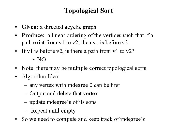
Topological Sort • Given: a directed acyclic graph • Produce: a linear ordering of the vertices such that if a path exist from v 1 to v 2, then v 1 is before v 2. • If v 1 is before v 2, is there a path from v 1 to v 2? • NO • Note: there may be multiple correct topological sorts • Algorithm Idea: – any vertex with indegree 0 can be first – Output and delete that vertex – update indegree’s of its sons – Repeat until empty • So we need to compute and keep track of indegree’s

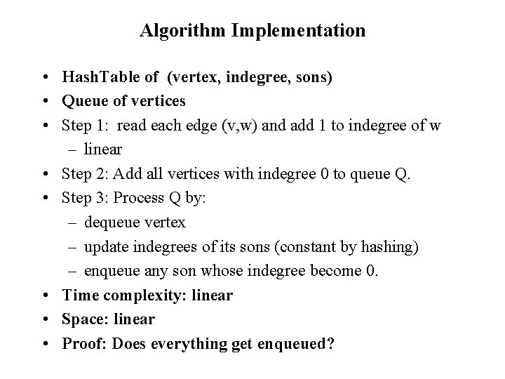
Algorithm Implementation • Hash. Table of (vertex, indegree, sons) • Queue of vertices • Step 1: read each edge (v, w) and add 1 to indegree of w – linear • Step 2: Add all vertices with indegree 0 to queue Q. • Step 3: Process Q by: – dequeue vertex – update indegrees of its sons (constant by hashing) – enqueue any son whose indegree become 0. • Time complexity: linear • Space: linear • Proof: Does everything get enqueued?

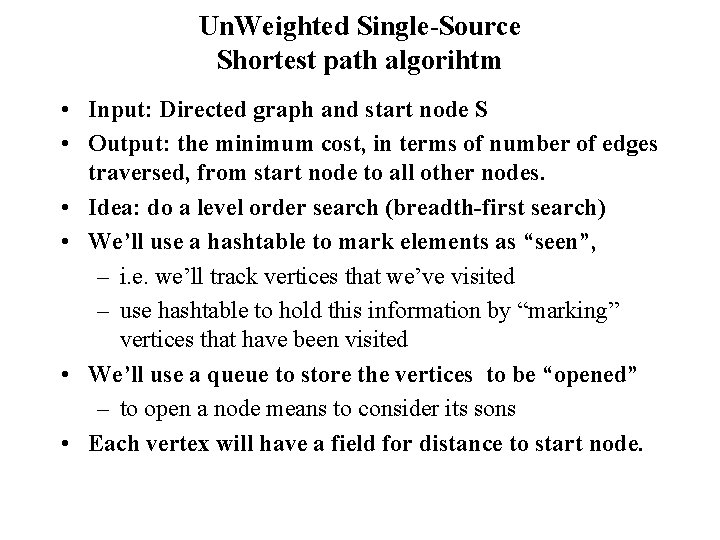
Un. Weighted Single-Source Shortest path algorihtm • Input: Directed graph and start node S • Output: the minimum cost, in terms of number of edges traversed, from start node to all other nodes. • Idea: do a level order search (breadth-first search) • We’ll use a hashtable to mark elements as “seen”, – i. e. we’ll track vertices that we’ve visited – use hashtable to hold this information by “marking” vertices that have been visited • We’ll use a queue to store the vertices to be “opened” – to open a node means to consider its sons • Each vertex will have a field for distance to start node.

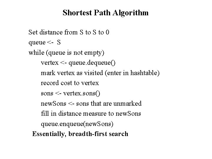
Shortest Path Algorithm Set distance from S to 0 queue <- S while (queue is not empty) vertex <- queue. dequeue() mark vertex as visited (enter in hashtable) record cost to vertex sons <- vertex. sons() new. Sons <- sons that are unmarked fill in distance measure to new. Sons queue. enqueue(new. Sons) Essentially, breadth-first search

Discussion • Will this terminate? – Will we ever revisit a node? • Computational cost? – O(|E|) • What are the memory requirements? – Suppose we don’t count graph (virtual graphs) – Can we bound queue? – Only O(|E|) and if m-ary tree, this is exponential. • Did we need the hashtable? – This avoids a linear search of the constructed graph – remove a factor of O(|G|).

Positive-Weighted Single-source Cheapest Path • Suppose we have positive costs associated with every edge in a directed graph. • Problem: Find the shortest path(total cost) from given vertex S to every vertex. • Solution: Dijstra’s algorithm • BFS idea still works, with slight modifications – Replace Queue by Priority queue. – As before, replace new. Sons by better. Sons. – As before, replace add entry to update entry (which may be add) – Note: may reopen an old son( if return with better path) • Dense graphs: O(|V|^2), sparse graphs: O(|E|log|V|)

Weighted Shortest Path Pseudo-Code Set distance from S to 0 (on node) Priority Queue PQ <- S while (PQ is not empty) vertex <- PQ. dequeue() … remove min mark vertex as visited (enter in hashtable) record cost to vertex sons <- vertex. sons() good. Sons <- new sons OR old sons with better costs estimates queue. enqueue(good. Sons)… enqueue puts in proper order.

Graphs with negative edge costs • Dijsktra doesn’t work (since we may have cycles which lower the cost) • Input: Directed graph with arbitrary edge costs and vertex v. • Output: Minimum cost from S to every vertex OR graph has a negative cost cycle. • Note: If no negative cost cycles, then a vertex can be visited (expanded) at most |V| times. • Algorithm: Add counter to each vertex so each time it is visited with lower cost, counter goes up. If counter exceeds |V|, then graph has negative cost cycle and we exit. Otherwise queue will be empty.

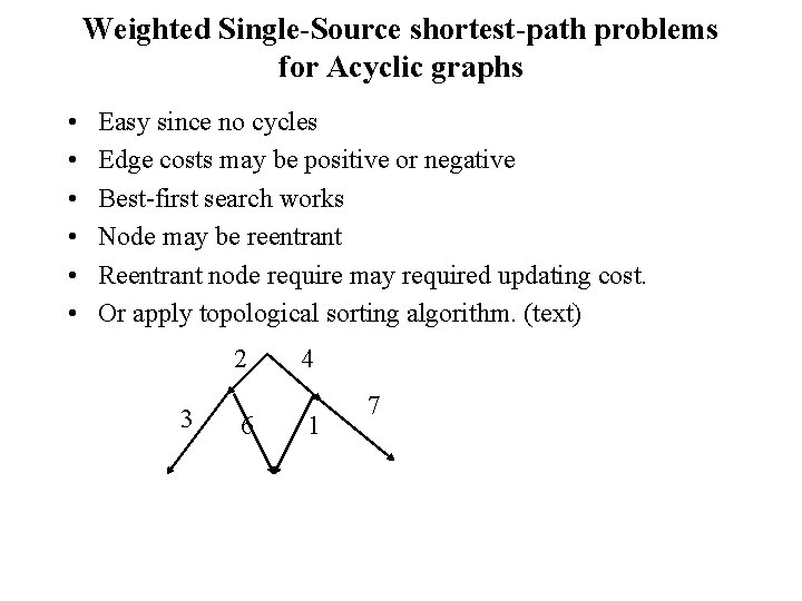
Weighted Single-Source shortest-path problems for Acyclic graphs • • • Easy since no cycles Edge costs may be positive or negative Best-first search works Node may be reentrant Reentrant node require may required updating cost. Or apply topological sorting algorithm. (text) 2 3 6 4 1 7

Algorithm Display • Idea: – Iterative use of breadth first search – addition of edges to effect other choices • See Diagrams provided • Analysis: (requires augmented path be cheapest) – Runs in linear time

Minimum Spanning Tree • Given: an undirected connected graph with edge costs • Output: a subtree of graph such that – contains all vertices – sum of costs of edges is minimum • If costs not given, assume 1. What then? – Note all spanning trees have same number of edges • Application: – Is undirected Graph with n vertices connected? • IFF minimal spanning tree has n-1 edges.

Prim’s Algorithm • • • Let G be given as (V, E) where V has n vertices Let T = empty Algorithm Idea: grow cheapest tree Choose a random v to start and add to T Repeat (until T has n vertices) – select edge of minimum length that does not form a cycle and that attaches to current tree (how to check? ) – add edge to T • The proof is more difficult than the code. • Complexity depends on G and code • O(V^2) for dense graphs • O(E*log(V)) for sparse graphs (use binary heap)

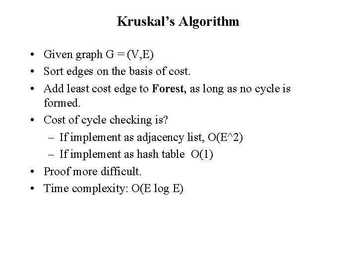
Kruskal’s Algorithm • Given graph G = (V, E) • Sort edges on the basis of cost. • Add least cost edge to Forest, as long as no cycle is formed. • Cost of cycle checking is? – If implement as adjacency list, O(E^2) – If implement as hash table O(1) • Proof more difficult. • Time complexity: O(E log E)

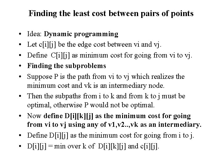
Finding the least cost between pairs of points • • • Idea: Dynamic programming Let c[i][j] be the edge cost between vi and vj. Define C[i][j] as minimum cost for going from vi to vj. Finding the subproblems Suppose P is the path from vi to vj which realizes the minimum cost and vk is an intermediary node. Then the subpaths from i to k and from k to j must be optimal, otherwise P would not be optimal. Now define D[i][k][j] as the minimum cost for going from vi to vj using any of v 1, v 2. . , vk as an intermediary. Define D[i][j] as the minimum cost for going from i to j. D[i][j] = min over k of D[i][k][j] and c[i][j].

All-Pairs (Floyd’s)Pseudo-Code • Initialization: – D[i][0][j] =cost(i, j) for all vertices i, j … O(|V|^2) – D[i][k+1][j] = • min(D[i][k][j], D[i][k][k+1]+D[k+1][k][j]) – This last statement is true since any path from the shortest path from vi to vj using {v 1, …vk+1} either doesn’t use vk+1, or the path divides into a path from vi to vk+1 and one from vk+1 to vj. • The cost of this is O(|V|^3) - i. e. single loop over all vertices with |V|^2 per loop.

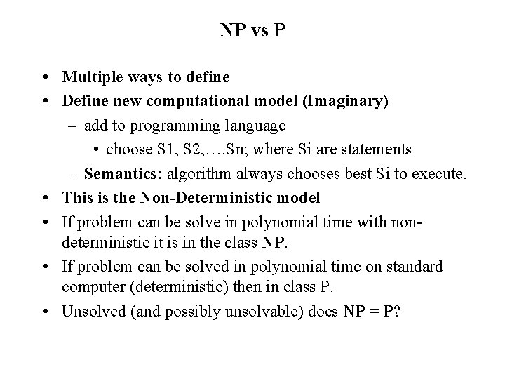
NP vs P • Multiple ways to define • Define new computational model (Imaginary) – add to programming language • choose S 1, S 2, …. Sn; where Si are statements – Semantics: algorithm always chooses best Si to execute. • This is the Non-Deterministic model • If problem can be solve in polynomial time with nondeterministic it is in the class NP. • If problem can be solved in polynomial time on standard computer (deterministic) then in class P. • Unsolved (and possibly unsolvable) does NP = P?

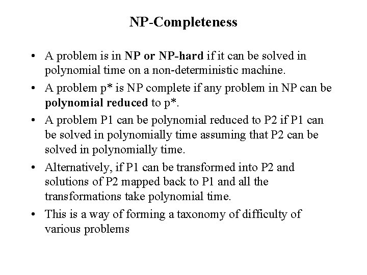
NP-Completeness • A problem is in NP or NP-hard if it can be solved in polynomial time on a non-deterministic machine. • A problem p* is NP complete if any problem in NP can be polynomial reduced to p*. • A problem P 1 can be polynomial reduced to P 2 if P 1 can be solved in polynomially time assuming that P 2 can be solved in polynomially time. • Alternatively, if P 1 can be transformed into P 2 and solutions of P 2 mapped back to P 1 and all the transformations take polynomial time. • This is a way of forming a taxonomy of difficulty of various problems

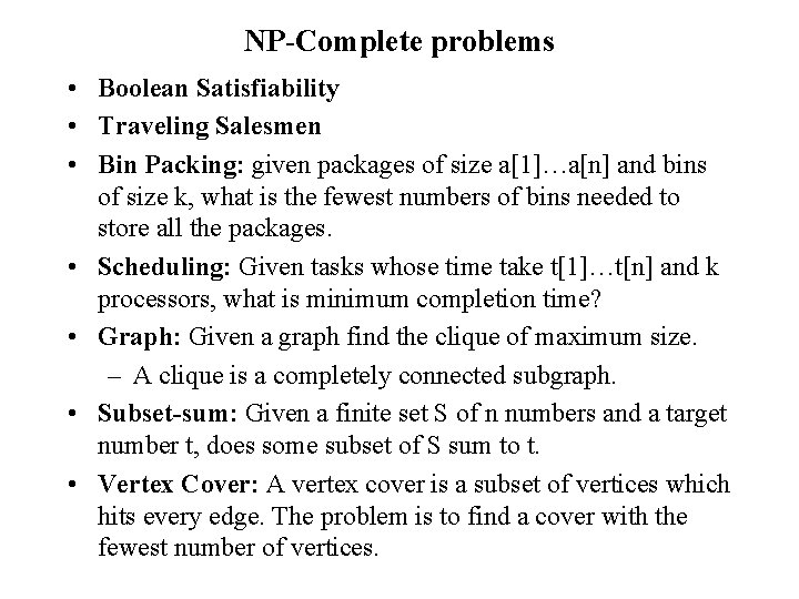
NP-Complete problems • Boolean Satisfiability • Traveling Salesmen • Bin Packing: given packages of size a[1]…a[n] and bins of size k, what is the fewest numbers of bins needed to store all the packages. • Scheduling: Given tasks whose time take t[1]…t[n] and k processors, what is minimum completion time? • Graph: Given a graph find the clique of maximum size. – A clique is a completely connected subgraph. • Subset-sum: Given a finite set S of n numbers and a target number t, does some subset of S sum to t. • Vertex Cover: A vertex cover is a subset of vertices which hits every edge. The problem is to find a cover with the fewest number of vertices.