Graphs 1 Chapter Outline Graph background and terminology

Graphs 1

Chapter Outline • • • Graph background and terminology Data structures for graphs Graph traversal algorithms Minimum spanning tree algorithms Shortest-path algorithm 2

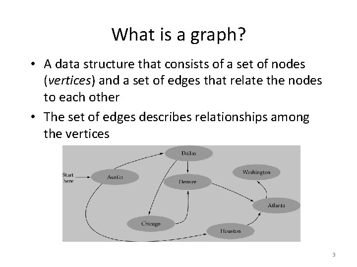
What is a graph? • A data structure that consists of a set of nodes (vertices) and a set of edges that relate the nodes to each other • The set of edges describes relationships among the vertices 3

Formal definition of graphs • A graph G is defined as follows: G=(V, E) V(G): a finite, nonempty set of vertices E(G): a set of edges (pairs of vertices) • V(G) and E(G) represent the sets of vertices and edges of G, respectively 4

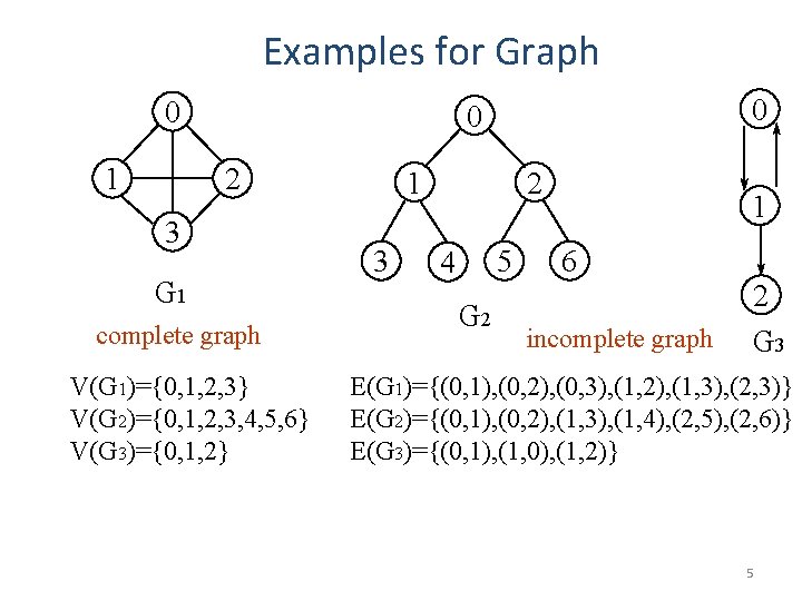
Examples for Graph 0 1 0 0 2 3 G 1 complete graph V(G 1)={0, 1, 2, 3} V(G 2)={0, 1, 2, 3, 4, 5, 6} V(G 3)={0, 1, 2} 1 3 2 5 4 G 2 1 6 incomplete graph 2 G 3 E(G 1)={(0, 1), (0, 2), (0, 3), (1, 2), (1, 3), (2, 3)} E(G 2)={(0, 1), (0, 2), (1, 3), (1, 4), (2, 5), (2, 6)} E(G 3)={(0, 1), (1, 0), (1, 2)} 5

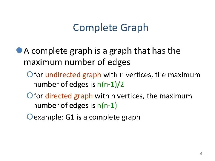
Complete Graph l A complete graph is a graph that has the maximum number of edges ¡for undirected graph with n vertices, the maximum number of edges is n(n-1)/2 ¡for directed graph with n vertices, the maximum number of edges is n(n-1) ¡example: G 1 is a complete graph 6

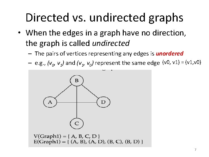
Directed vs. undirected graphs • When the edges in a graph have no direction, the graph is called undirected – The pairs of vertices representing any edges is unordered – e. g. , (v 0, v 1) and (v 1, v 0) represent the same edge (v 0, v 1) = (v 1, v 0) 7

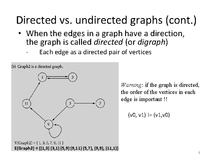
Directed vs. undirected graphs (cont. ) • When the edges in a graph have a direction, the graph is called directed (or digraph) - Each edge as a directed pair of vertices Warning: if the graph is directed, the order of the vertices in each edge is important !! (v 0, v 1) != (v 1, v 0) E(Graph 2) = {(1, 3) (3, 1) (5, 9) (9, 11) (5, 7), (9, 9), (11, 1)} 8

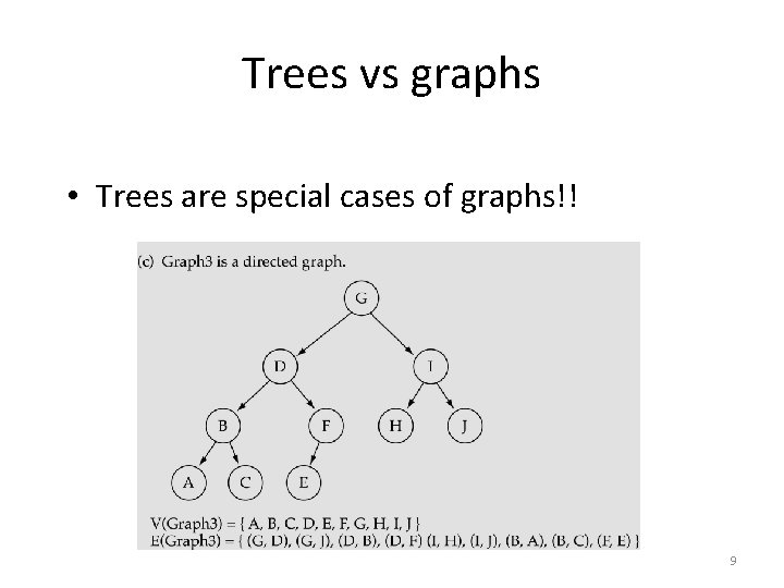
Trees vs graphs • Trees are special cases of graphs!! 9

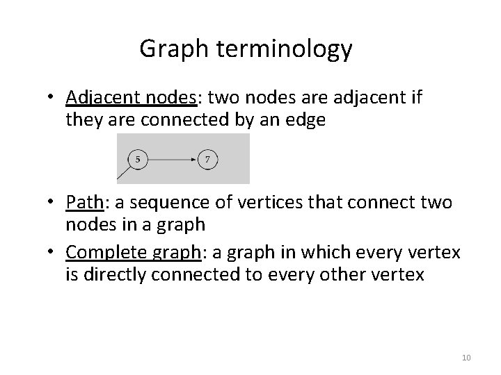
Graph terminology • Adjacent nodes: two nodes are adjacent if they are connected by an edge • Path: a sequence of vertices that connect two nodes in a graph • Complete graph: a graph in which every vertex is directly connected to every other vertex 10

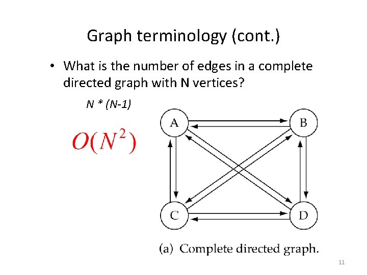
Graph terminology (cont. ) • What is the number of edges in a complete directed graph with N vertices? N * (N-1) 11

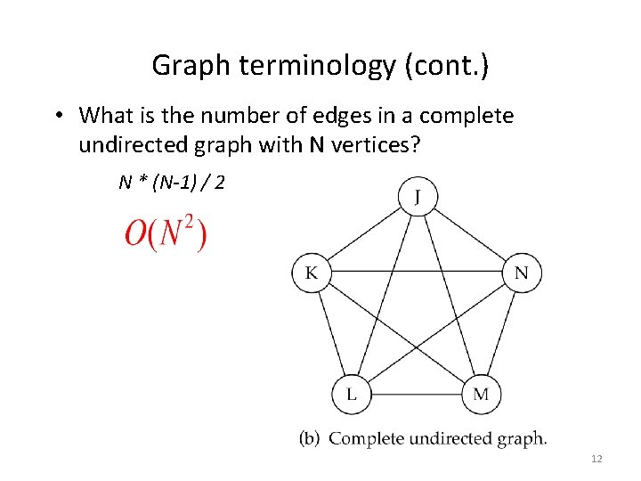
Graph terminology (cont. ) • What is the number of edges in a complete undirected graph with N vertices? N * (N-1) / 2 12

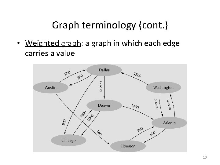
Graph terminology (cont. ) • Weighted graph: a graph in which each edge carries a value 13

Data Structures for Graphs an Adjacency Matrix • A two-dimensional matrix or array that has one row and one column for each node in the graph • For each edge of the graph (Vi, Vj), the location of the matrix at row i and column j is 1 • All other locations are 0 • For an undirected graph, the matrix will be symmetric along the diagonal • For a weighted graph, the adjacency matrix would have the weight for edges in the graph 14

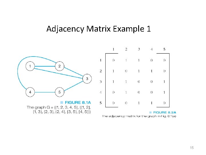
Adjacency Matrix Example 1 15

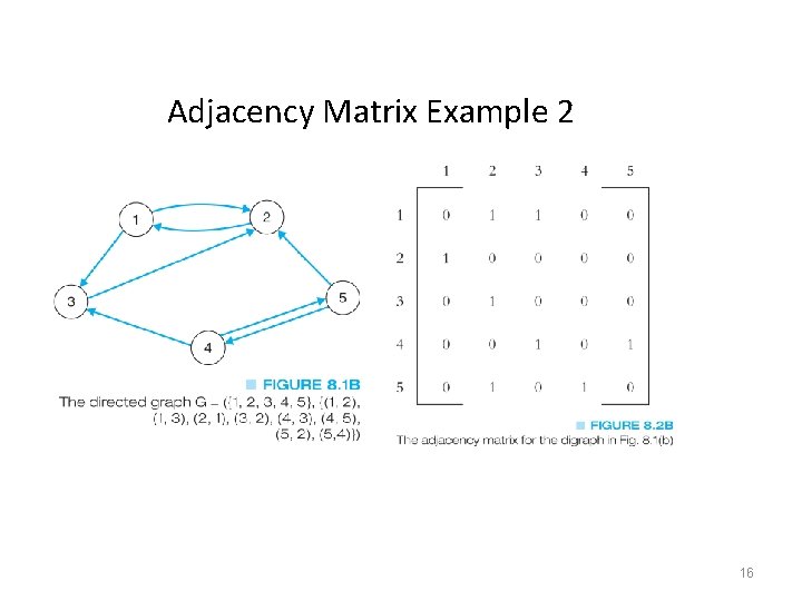
Adjacency Matrix Example 2 16

Data Structures for Graphs An Adjacency List • A list of pointers, one for each node of the graph • These pointers are the start of a linked list of nodes that can be reached by one edge of the graph • For a weighted graph, this list would also include the weight for each edge 17

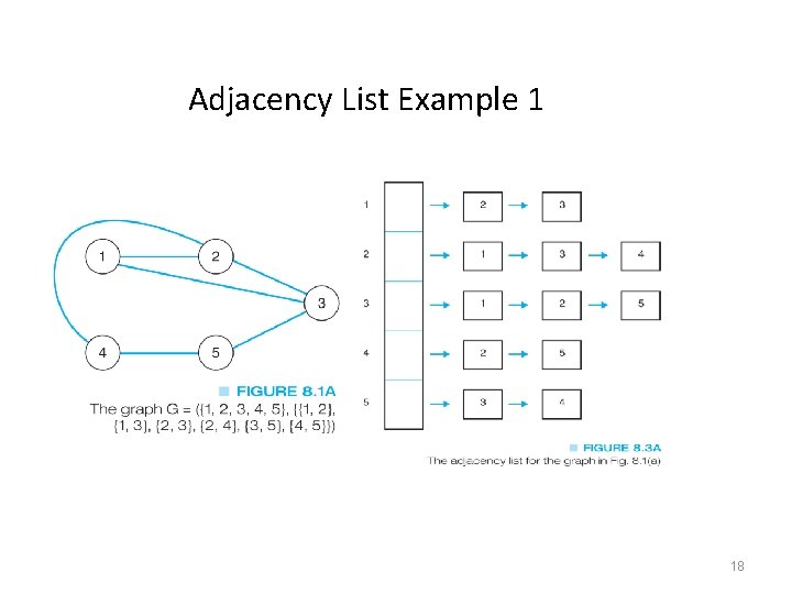
Adjacency List Example 1 18

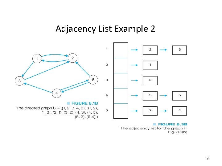
Adjacency List Example 2 19

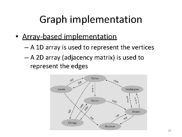
Graph implementation • Array-based implementation – A 1 D array is used to represent the vertices – A 2 D array (adjacency matrix) is used to represent the edges 20

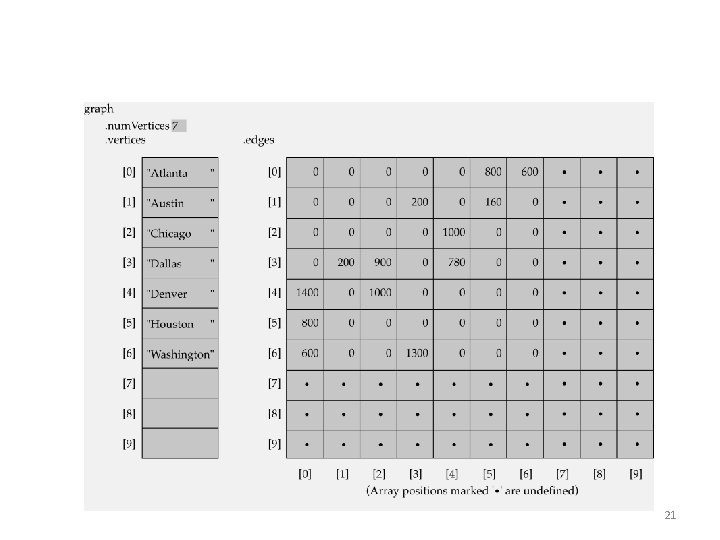
Array-based implementation 21

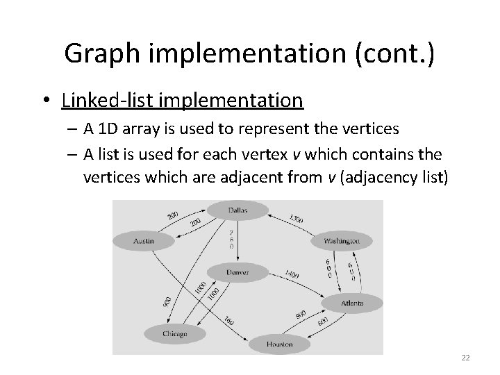
Graph implementation (cont. ) • Linked-list implementation – A 1 D array is used to represent the vertices – A list is used for each vertex v which contains the vertices which are adjacent from v (adjacency list) 22

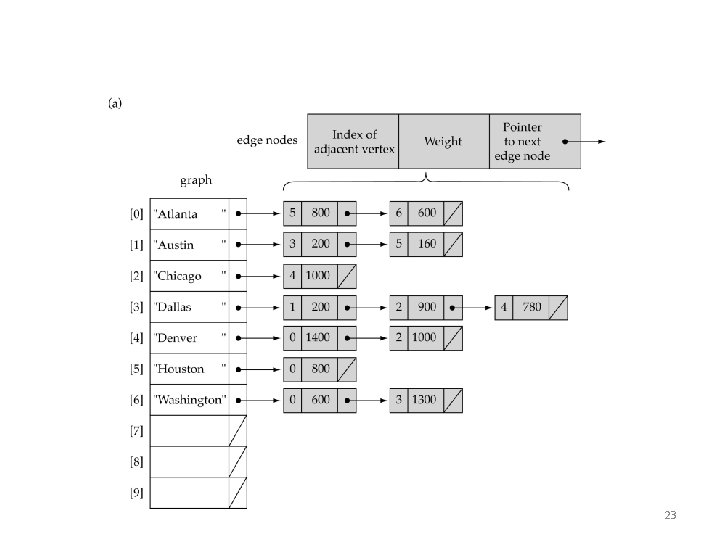
Linked-list implementation 23

Adjacency matrix vs. adjacency list representation • Adjacency matrix – Good for dense graphs – Memory requirements: O(V 2 ) – Connectivity between two vertices can be tested quickly • Adjacency list – Good for sparse graphs – Memory requirements: O(V + E)=O(V) – Vertices adjacent to another vertex can be found quickly 24

Graph searching • Problem: find a path between two nodes of the graph (e. g. , Austin and Washington) • Methods: Depth-First-Search (DFS) or Breadth-First-Search (BFS) 25

Depth-First-Search (DFS) • What is the idea behind DFS? – Travel as far as you can down a path – Back up as little as possible when you reach a "dead end" (i. e. , next vertex has been "marked" or there is no next vertex) • DFS can be implemented efficiently using a stack 26

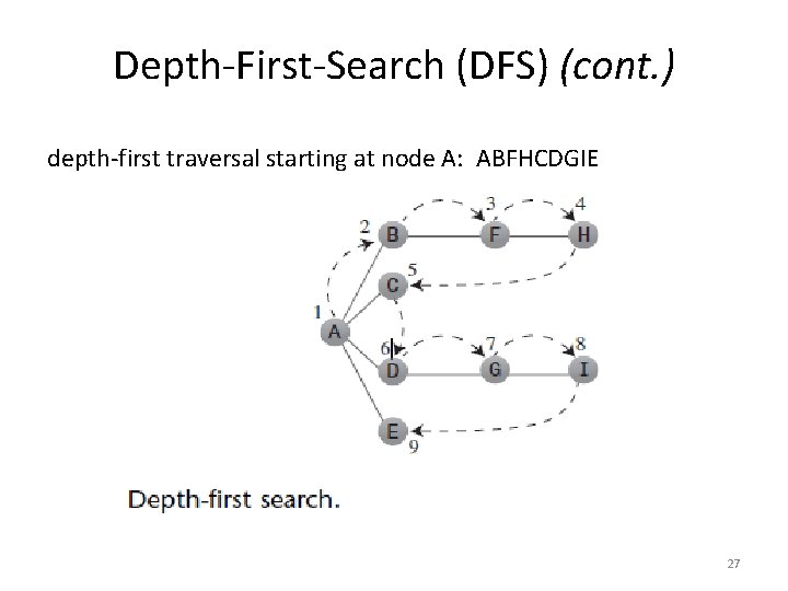
Depth-First-Search (DFS) (cont. ) depth-first traversal starting at node A: ABFHCDGIE 27

Depth-First-Search (DFS) (cont. ) • Pick a starting point— say A. • Then do 3 things: visit this vertex, push it onto a stack so you can remember it, and mark it so you won’t visit it again. • Next, go to any vertex adjacent to A that hasn’t yet been visited. say B. Visit B, mark it, and push it on the stack. • At B, repeat as before: this process is Rule 1. RULE 1 • If possible, visit an adjacent unvisited vertex, mark it, and push it on the stack. RULE 2 • If you can’t follow Rule 1, then, if possible, pop a vertex off the stack. RULE 3 • If you can’t follow Rule 1 or Rule 2, you’re done. 28

Breadth-First-Searching (BFS) • What is the idea behind BFS? – Look at all possible paths at the same depth before you go at a deeper level – Back up as far as possible when you reach a "dead end" (i. e. , next vertex has been "marked" or there is no next vertex) 31

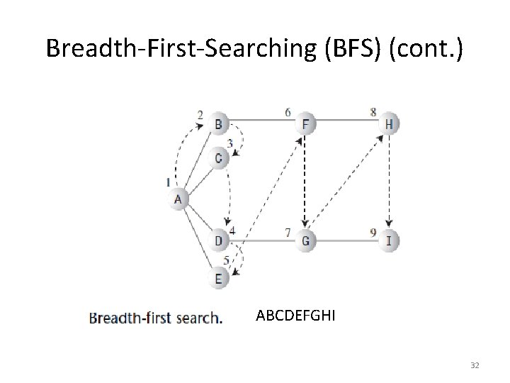
Breadth-First-Searching (BFS) (cont. ) ABCDEFGHI 32

Breadth-First-Searching (BFS) (cont. ) Pick a starting point— say A. RULE 1 • Visit the next unvisited vertex (if there is one) that’s adjacent to the current vertex, mark it, and insert it into the queue. RULE 2 • If you can’t carry out Rule 1 because there are no more unvisited vertices, remove a vertex from the queue (if possible) and make it the current vertex. RULE 3 • If you can’t carry out Rule 2 because the queue is empty, you’re done 33

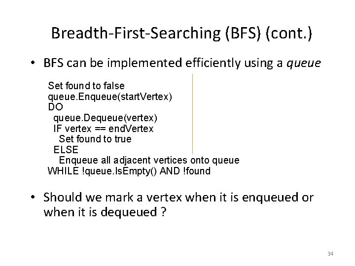
Breadth-First-Searching (BFS) (cont. ) • BFS can be implemented efficiently using a queue IF(!found) Set found to false Write "Path does not exist" queue. Enqueue(start. Vertex) DO queue. Dequeue(vertex) IF vertex == end. Vertex Set found to true ELSE Enqueue all adjacent vertices onto queue WHILE !queue. Is. Empty() AND !found • Should we mark a vertex when it is enqueued or when it is dequeued ? 34

Breadth-First Traversal • From the starting node, follow all paths of length one • Then follow paths of length two that go to unvisited nodes • Continue increasing the length of the paths until there are no unvisited nodes along any of the paths 35

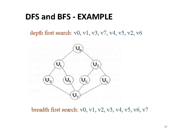
DFS and BFS - EXAMPLE depth first search: v 0, v 1, v 3, v 7, v 4, v 5, v 2, v 6 breadth first search: v 0, v 1, v 2, v 3, v 4, v 5, v 6, v 7 37

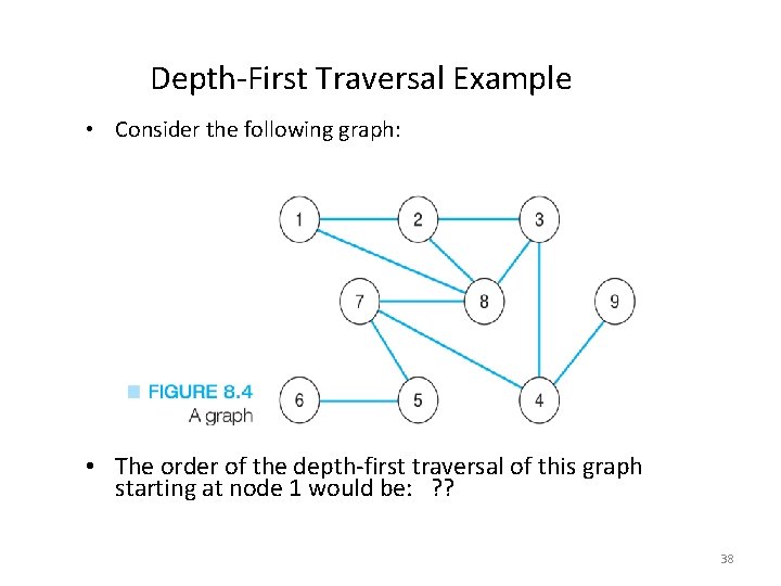
Depth-First Traversal Example • Consider the following graph: • The order of the depth-first traversal of this graph starting at node 1 would be: ? ? 38

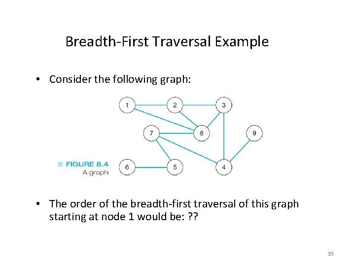
Breadth-First Traversal Example • Consider the following graph: • The order of the breadth-first traversal of this graph starting at node 1 would be: ? ? 39

Traversal Analysis • If the graph is connected, these methods will visit each node exactly once • Because the most complex work is done when the node is visited, we can consider these to be O(N) • If we count the number of edges considered, we will find that is also linear with respect to the number of graph edges 40

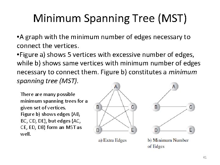
Minimum Spanning Tree (MST) • A graph with the minimum number of edges necessary to connect the vertices. • Figure a) shows 5 vertices with excessive number of edges, while b) shows same vertices with minimum number of edges necessary to connect them. Figure b) constitutes a minimum spanning tree (MST). There are many possible minimum spanning trees for a given set of vertices. Figure b) shows edges {AB, BC, CD, DE}, but edges {AC, CE, ED, DB} form an MST as well. 41

Minimum Spanning Tree (MST) • The number of edges E in an MST is always one less than the number of vertices V: E=V– 1 • Remember we’re not trying to find a minimum physical length, just the minimum number of edges. • The algorithm for creating the minimum spanning tree is almost identical to the depth-first search or the breadth first search algorithms. 42

Minimum Spanning Tree with Weighted Graphs • The minimum spanning tree (MST) of a weighted connected graph is a subgraph that contains all of the nodes of the original graph and a subset of the edges so that: – The subgraph is connected – The total weights of the subgraph edges is the smallest possible 43

The Dijkstra-Prim Method • This is a greedy algorithm that solves the larger problem by looking at a subset and making the best choice for it • In this case, we will look at all of the edges from the starting node and choose the smallest • On each pass, we will choose the smallest of the edges from nodes already in the MST to nodes not in the MST (the fringe) 44

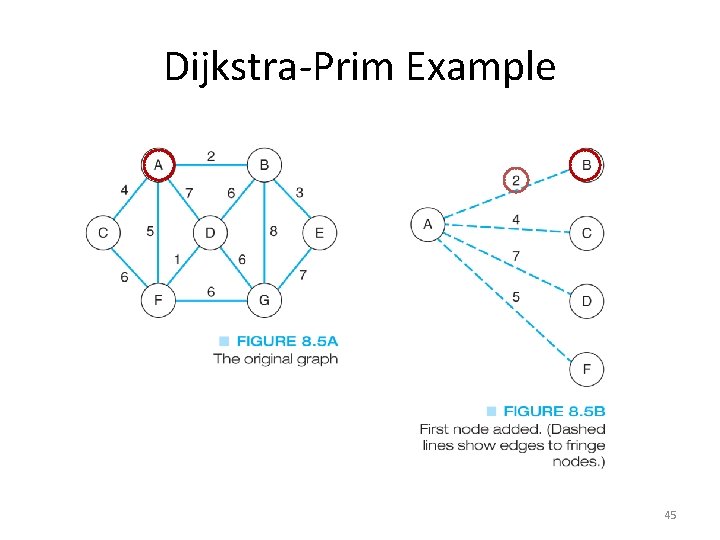
Dijkstra-Prim Example 45

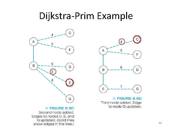
Dijkstra-Prim Example 46

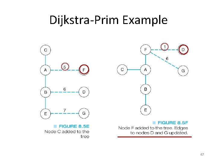
Dijkstra-Prim Example 47

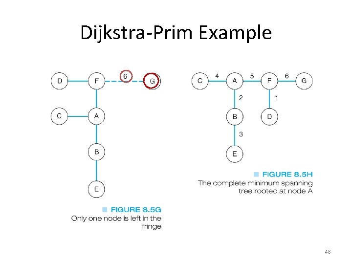
Dijkstra-Prim Example 48

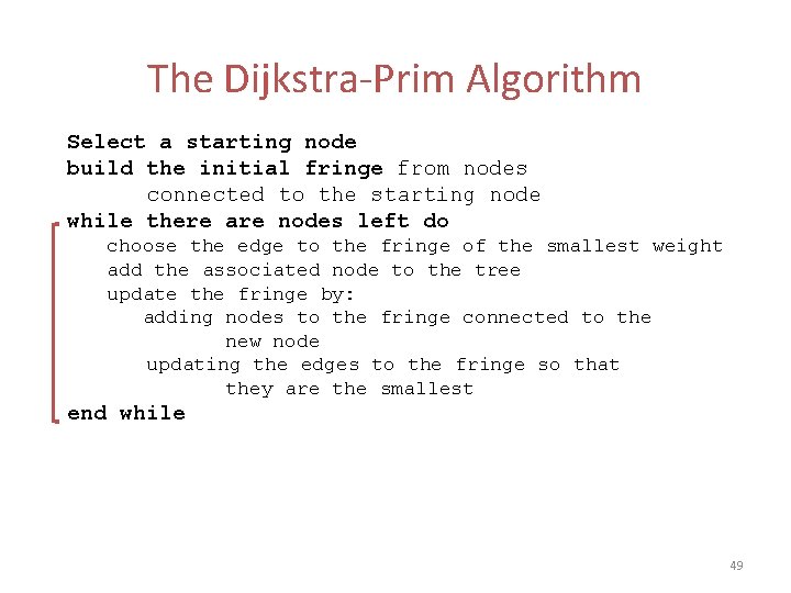
The Dijkstra-Prim Algorithm Select a starting node build the initial fringe from nodes connected to the starting node while there are nodes left do choose the edge to the fringe of the smallest weight add the associated node to the tree update the fringe by: adding nodes to the fringe connected to the new node updating the edges to the fringe so that they are the smallest end while 49

Shortest-Path Algorithm • The shortest-path algorithm finds the series of edges between two nodes that has the smallest total weight 50

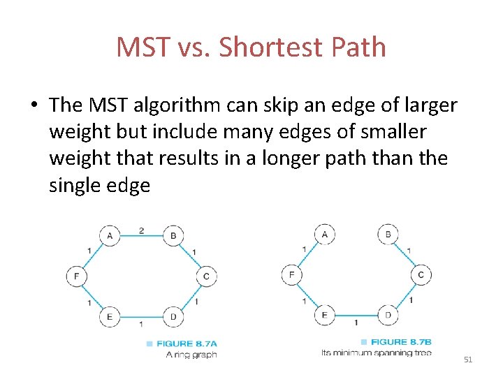
MST vs. Shortest Path • The MST algorithm can skip an edge of larger weight but include many edges of smaller weight that results in a longer path than the single edge 51

Shortest-path problem • There are multiple paths from a source vertex to a destination vertex • Shortest path: the path whose total weight (i. e. , sum of edge weights) is minimum • Common algorithms: Dijkstra's algorithm, Bellman-Ford algorithm • BFS can be used to solve the shortest path problem when the graph is weightless or all the weights are the same 52

Dijkstra’s Method • This is similar to the Dijkstra-Prim MST algorithm, but instead of just looking at the single shortest edge from a node to the fringe, we look at the shortest path from the start node to a fringe node 53

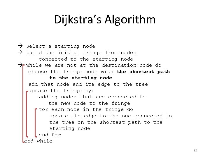
Dijkstra’s Algorithm Select a starting node build the initial fringe from nodes connected to the starting node while we are not at the destination node do choose the fringe node with the shortest path to the starting node add that node and its edge to the tree update the fringe by: adding nodes that are connected to the new node to the fringe for each node in the fringe do update its edge to the one connected to the tree on the shortest path to the starting node end for end while 54

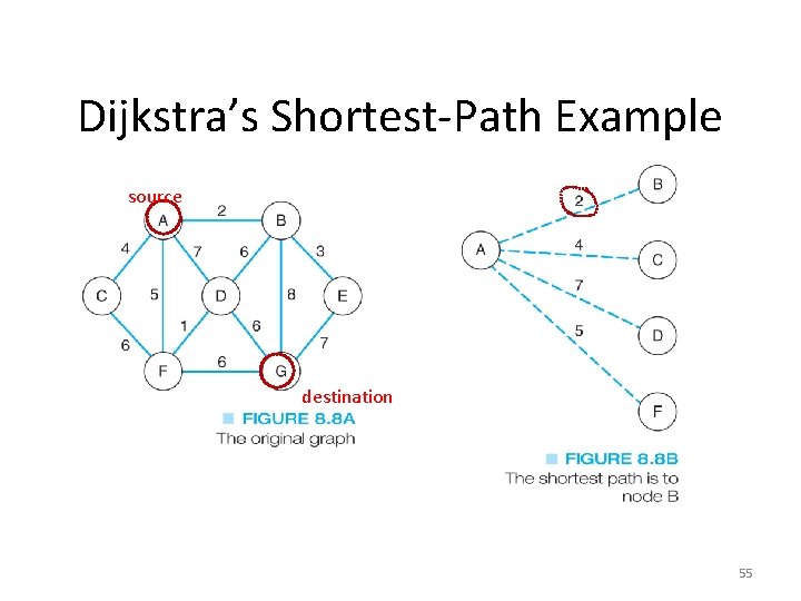
Dijkstra’s Shortest-Path Example source destination 55

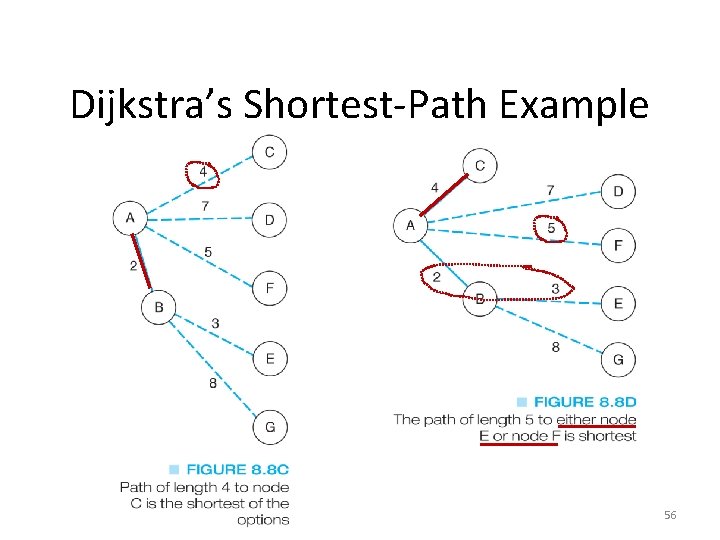
Dijkstra’s Shortest-Path Example 56

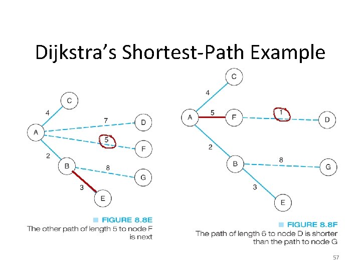
Dijkstra’s Shortest-Path Example 57

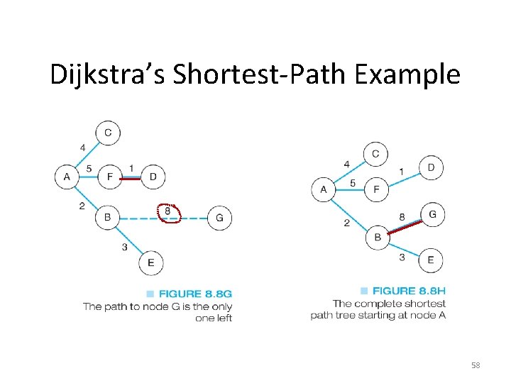
Dijkstra’s Shortest-Path Example 58

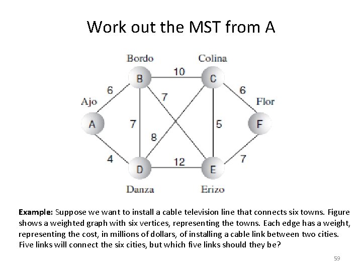
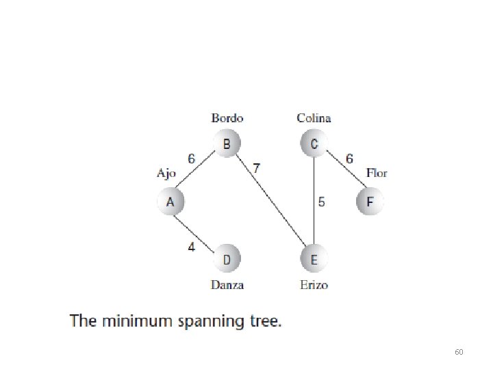
Work out the MST from A Example: Suppose we want to install a cable television line that connects six towns. Figure shows a weighted graph with six vertices, representing the towns. Each edge has a weight, representing the cost, in millions of dollars, of installing a cable link between two cities. Five links will connect the six cities, but which five links should they be? 59

60

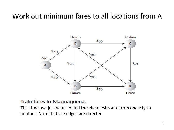
Work out minimum fares to all locations from A This time, we just want to find the cheapest route from one city to another. Note that the edges are directed 61

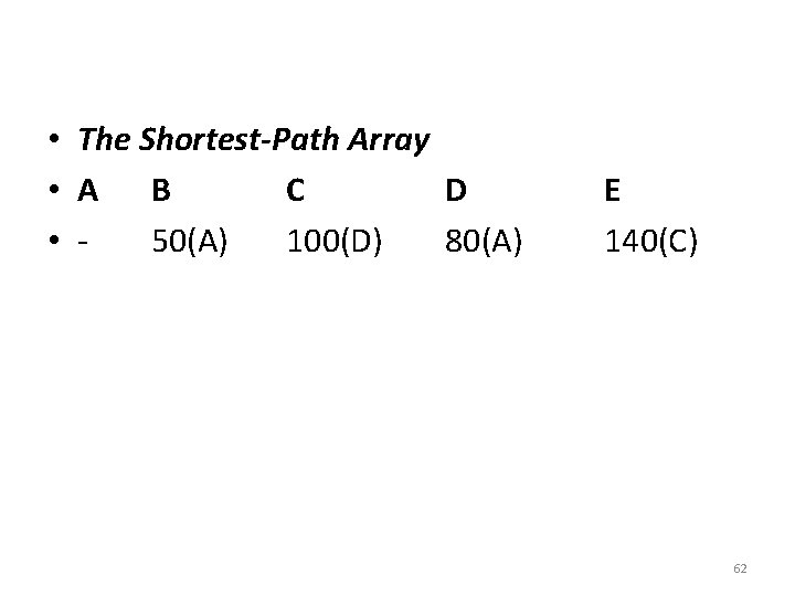
• The Shortest-Path Array • A B C D • 50(A) 100(D) 80(A) E 140(C) 62

Efficiency • • The issue is complicated by the two ways of representing graphs: the adjacency matrix and adjacency lists. If an adjacency matrix is used, the algorithms mostly require O(V 2) time, where V is the number of vertices. For large matrices, O(V 2) isn’t very good performance. If the graph is dense, there isn’t much we can do about improving this performance. (By dense we mean a graph that has many edges—one in which many or most of the cells in the adjacency matrix are filled. ) However, many graphs are sparse. In a sparse graph, running times can be improved by using the adjacency-list representation rather than the adjacency matrix. - You don’t waste time examining adjacency-matrix cells that don’t hold edges. For unweighted graphs, depth-first search with adjacency lists requires O(V+E) time For weighted graphs, both the minimum spanning tree and the shortest-path algorithm require O((E+V)log. V) time. In large sparse graphs, these times can represent dramatic improvements over the adjacency matrix approach. However, the algorithms are somewhat more complicated 64