Graphpad Prism 2 Session 2 2 way ANOVA

Graphpad Prism 2

Session 2 • • 2 -way ANOVA Mixed ANOVA Regression (simple and multiple) Pearson/Spearman correlation coefficient.

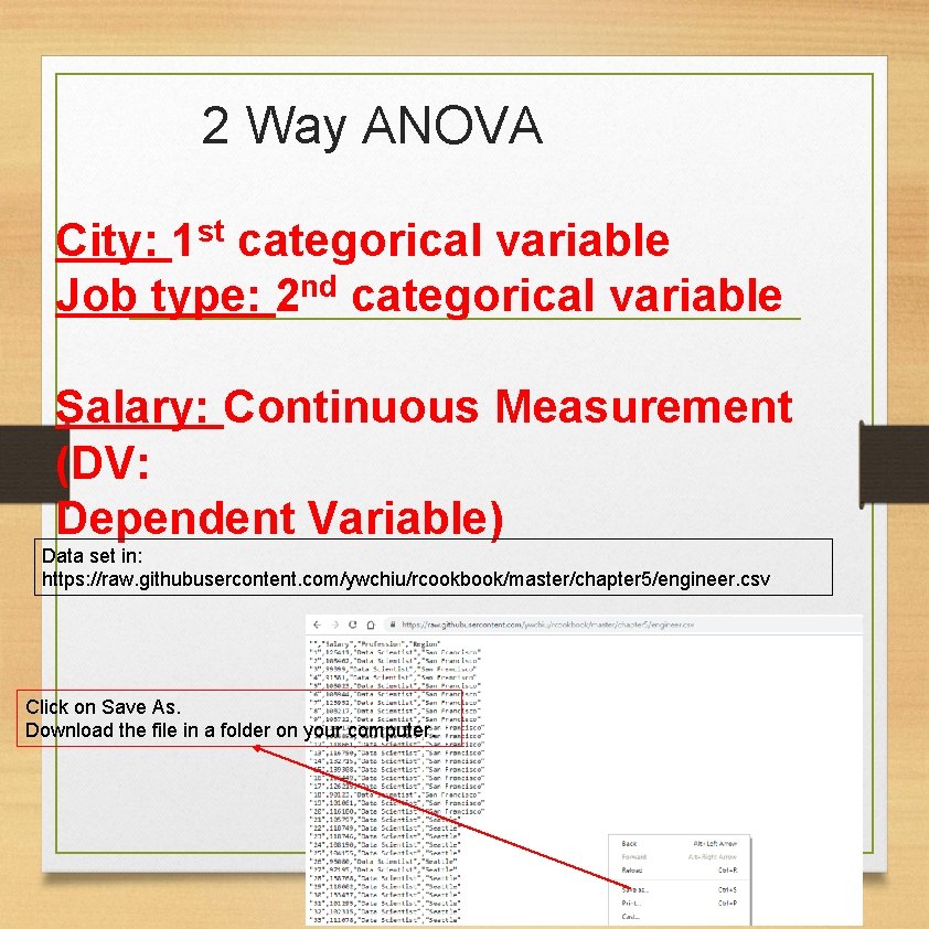
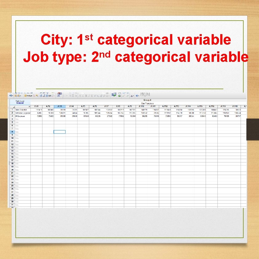
2 Way ANOVA City: 1 st categorical variable Job type: 2 nd categorical variable Salary: Continuous Measurement (DV: Dependent Variable) Data set in: https: //raw. githubusercontent. com/ywchiu/rcookbook/master/chapter 5/engineer. csv Click on Save As. Download the file in a folder on your computer.

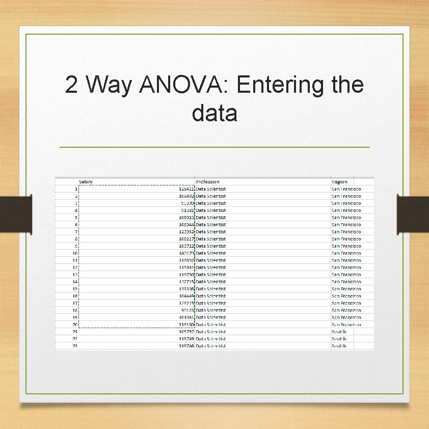
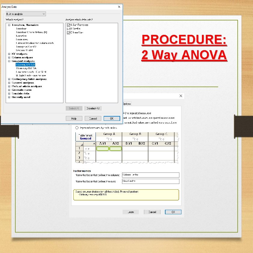
2 Way ANOVA: Entering the data

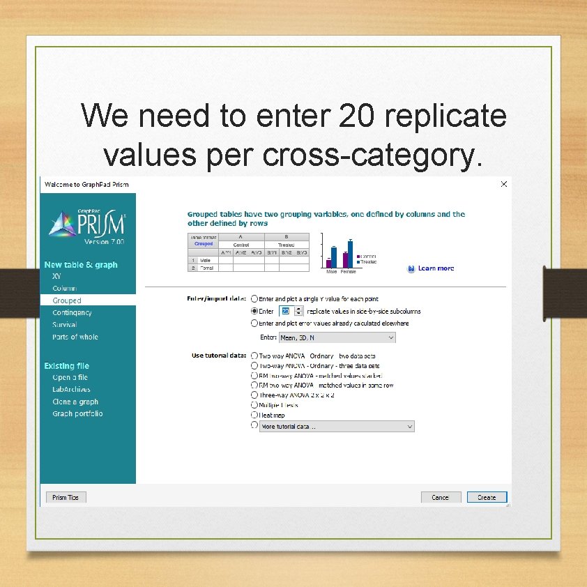
We need to enter 20 replicate values per cross-category.

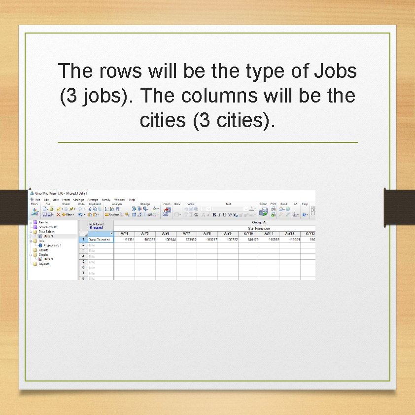
The rows will be the type of Jobs (3 jobs). The columns will be the cities (3 cities).

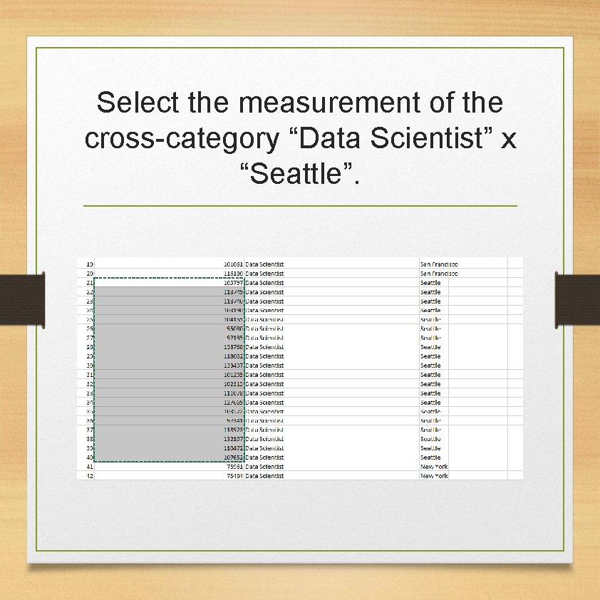
Select the measurement of the cross-category “Data Scientist” x “Seattle”.

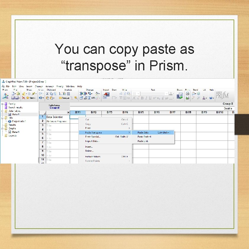
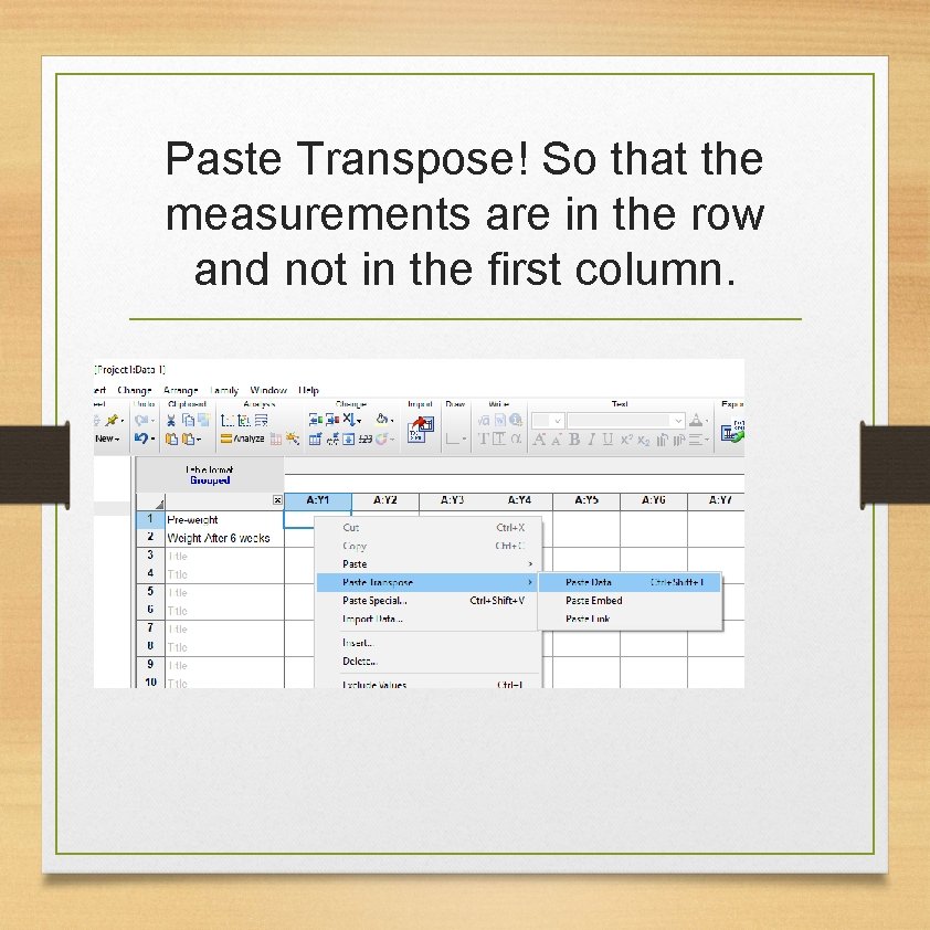
You can copy paste as “transpose” in Prism.

st 1 City: categorical variable nd Job type: 2 categorical variable

PROCEDURE: 2 Way ANOVA

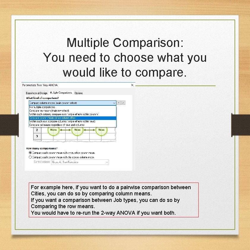
Multiple Comparison: You need to choose what you would like to compare. For example here, if you want to do a pairwise comparison between Cities, you can do so by comparing column means. If you want a comparison between Job types, you can do so by Comparing the row means. You would have to re-run the 2 -way ANOVA if you want both.

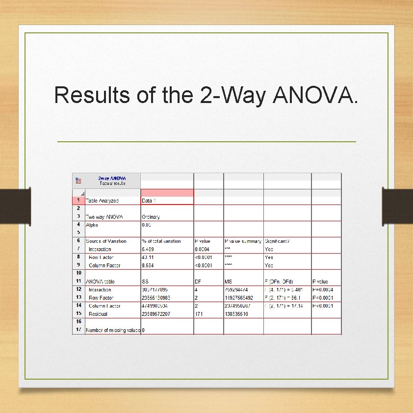
Results of the 2 -Way ANOVA.

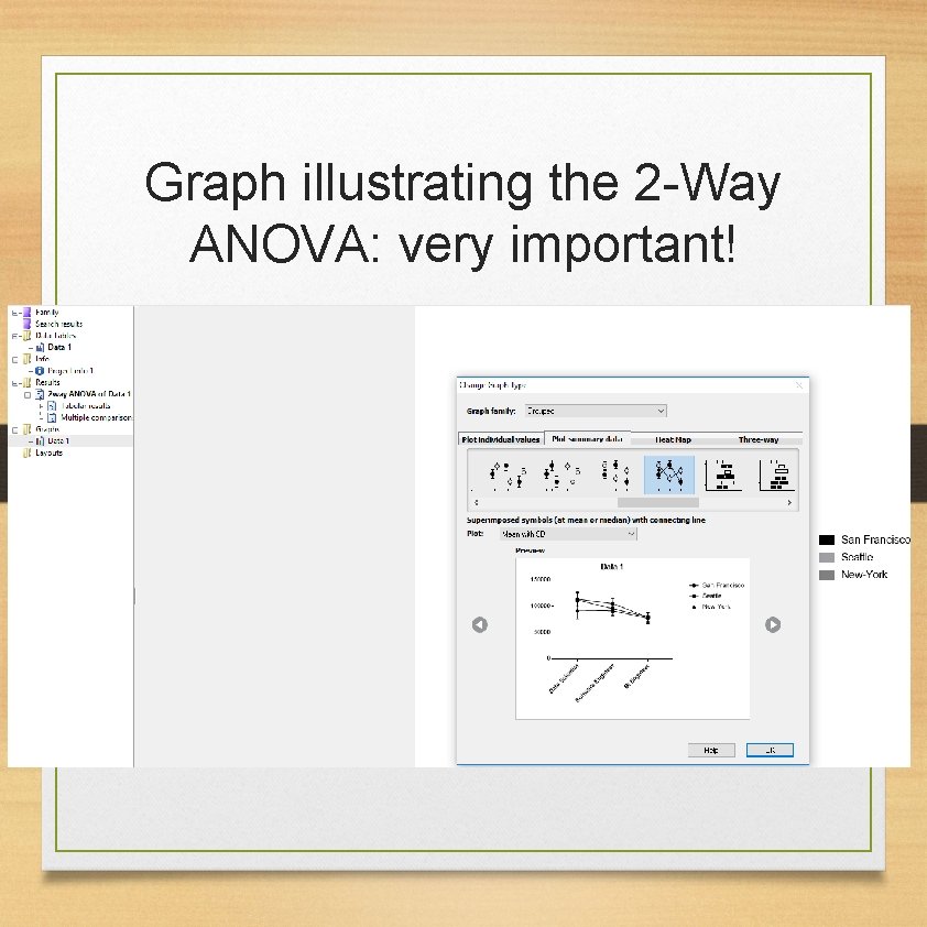
Graph illustrating the 2 -Way ANOVA: very important!

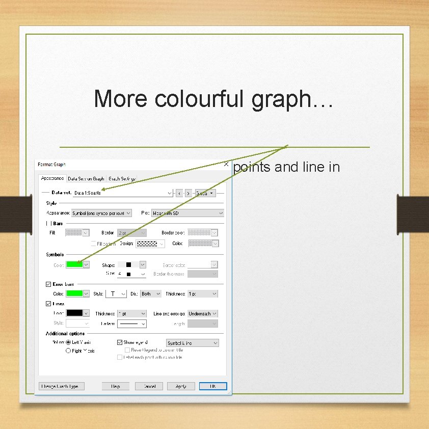
More colourful graph… • By Clicking on “Change”, symbol “histograms”, you can change the design. Here. We change the colour of San Francisco to Orange.

More colourful graph… • For Seattle, I can put the points and line in Green.

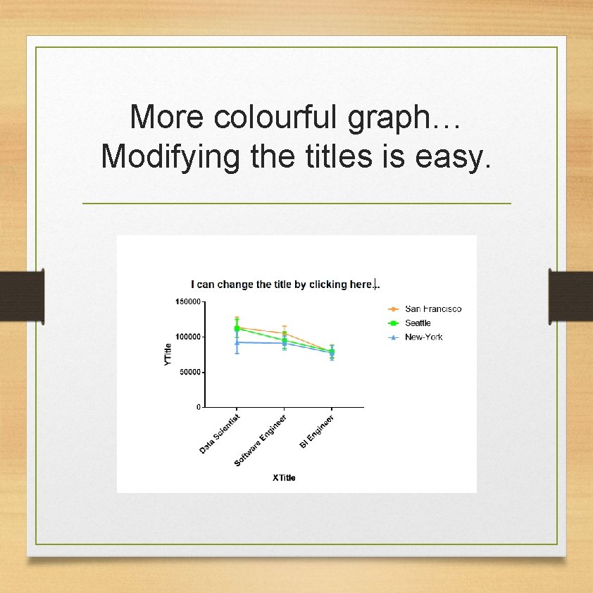
More colourful graph… Modifying the titles is easy.

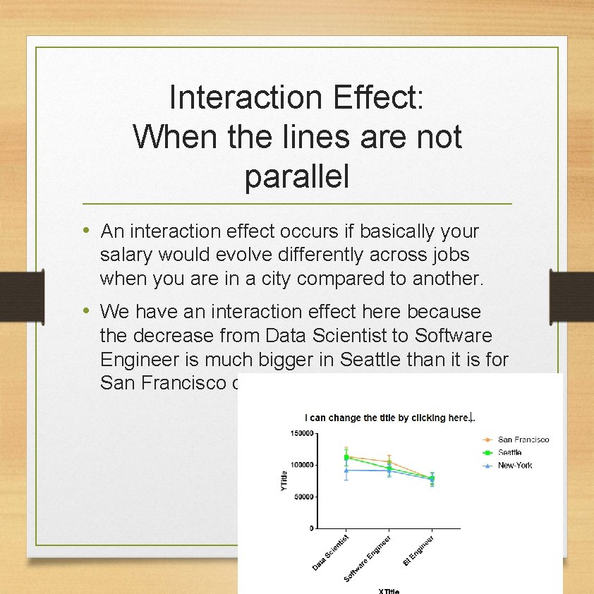
Interaction Effect: When the lines are not parallel • An interaction effect occurs if basically your salary would evolve differently across jobs when you are in a city compared to another. • We have an interaction effect here because the decrease from Data Scientist to Software Engineer is much bigger in Seattle than it is for San Francisco or New-York.

Mixed ANOVA: • Continuous variable/measurement: Diet group. • One categorical variable: Fixed Factor(at least 2 groups)= Between Factor. • At least 2 different times: Within-Factor • Basically the same as the 2 -Way ANOVA, but imagine instead of types of job you have 3 different times: 2009, 2014 and 2019. • You would have to study the effect across time, between groups and the interaction effect. • Download the Diet Data set (csv) from MASH website: https: //www. sheffield. ac. uk/mash/statistics/datas ets

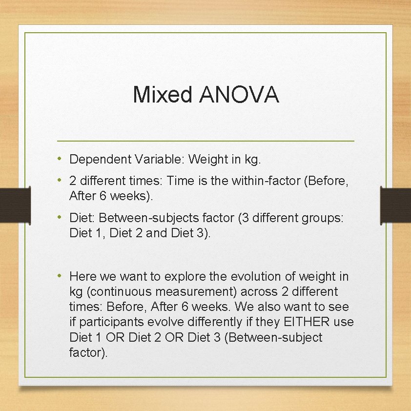
Mixed ANOVA • Dependent Variable: Weight in kg. • 2 different times: Time is the within-factor (Before, After 6 weeks). • Diet: Between-subjects factor (3 different groups: Diet 1, Diet 2 and Diet 3). • Here we want to explore the evolution of weight in kg (continuous measurement) across 2 different times: Before, After 6 weeks. We also want to see if participants evolve differently if they EITHER use Diet 1 OR Diet 2 OR Diet 3 (Between-subject factor).

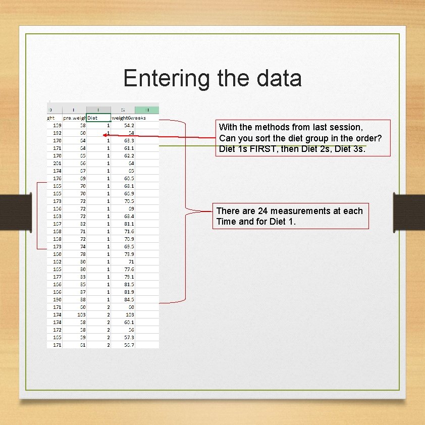
Entering the data With the methods from last session, Can you sort the diet group in the order? Diet 1 s FIRST, then Diet 2 s, Diet 3 s. There are 24 measurements at each Time and for Diet 1.

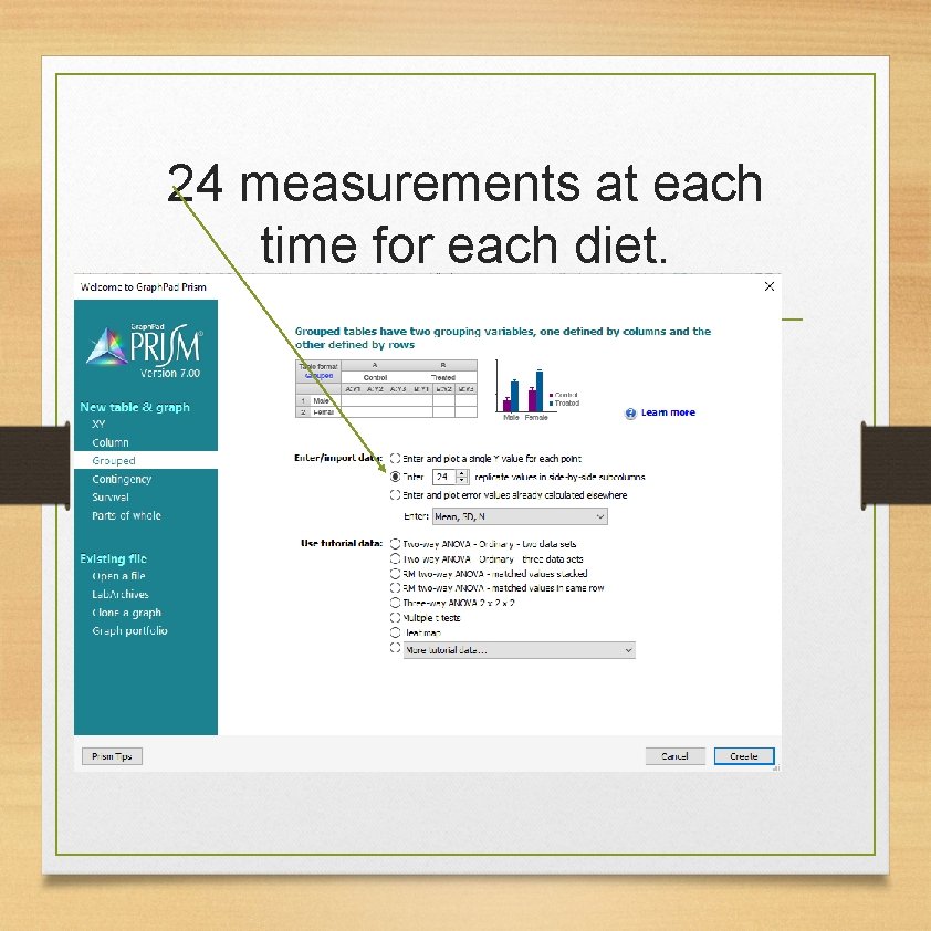
24 measurements at each time for each diet.

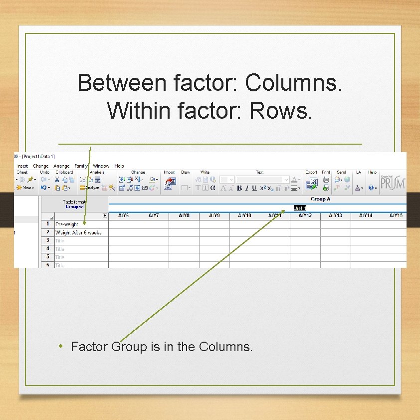
Between factor: Columns. Within factor: Rows. • Factor Time is in the Rows. • Factor Group is in the Columns.

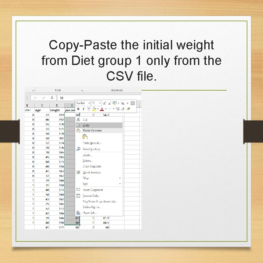
Copy-Paste the initial weight from Diet group 1 only from the CSV file.

Paste Transpose! So that the measurements are in the row and not in the first column.

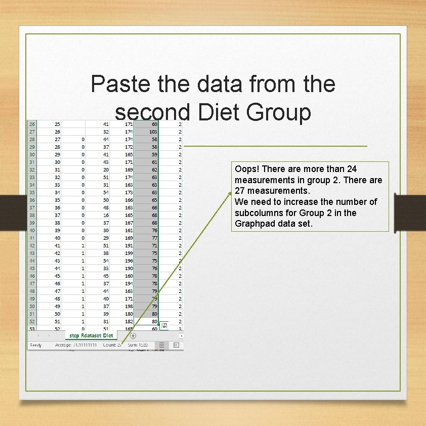
Paste the data from the second Diet Group Oops! There are more than 24 measurements in group 2. There are 27 measurements. We need to increase the number of subcolumns for Group 2 in the Graphpad data set.

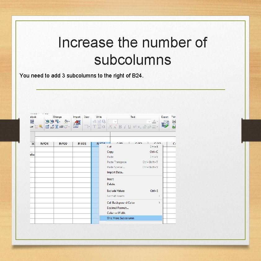
Increase the number of subcolumns You need to add 3 subcolumns to the right of B 24.

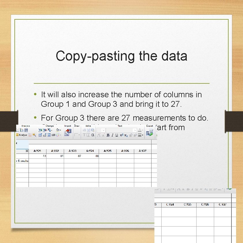
Copy-pasting the data • It will also increase the number of columns in Group 1 and Group 3 and bring it to 27. • For Group 3 there are 27 measurements to do. So there is nothing else to do apart from copying pasting the data.

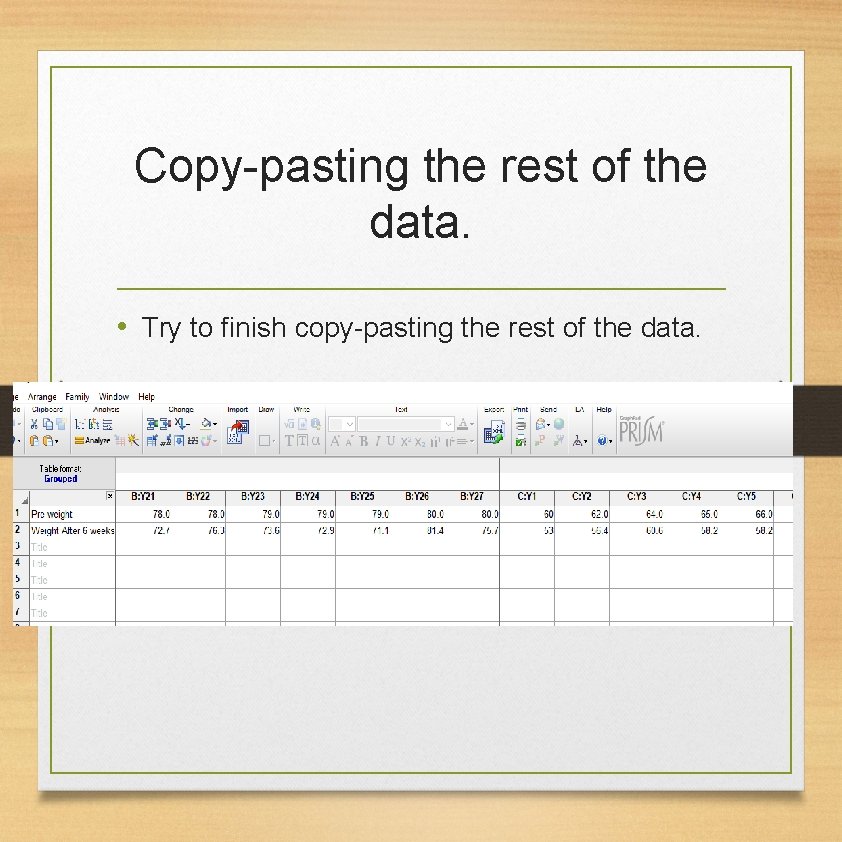
Copy-pasting the rest of the data. • Try to finish copy-pasting the rest of the data.

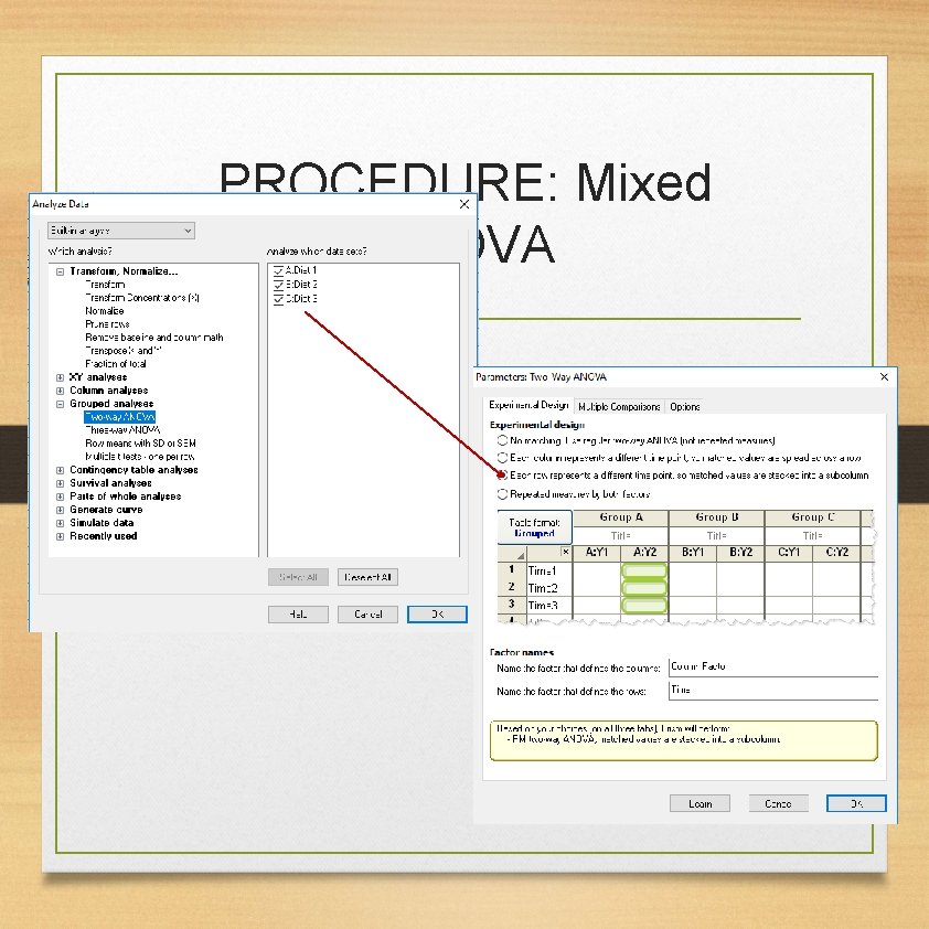
PROCEDURE: Mixed ANOVA

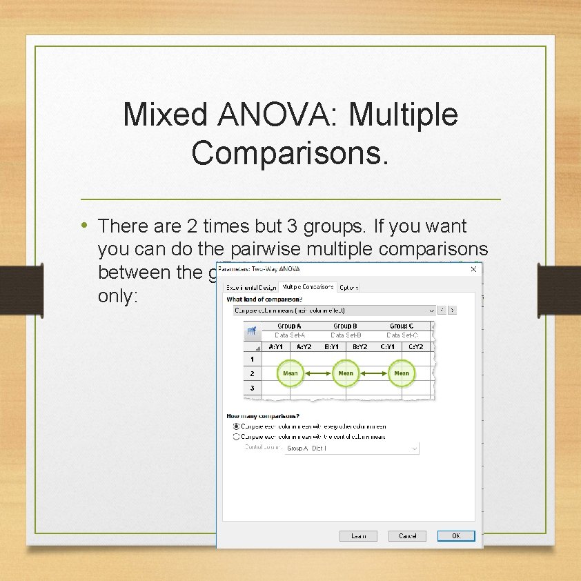
Mixed ANOVA: Multiple Comparisons. • There are 2 times but 3 groups. If you want you can do the pairwise multiple comparisons between the groups only:

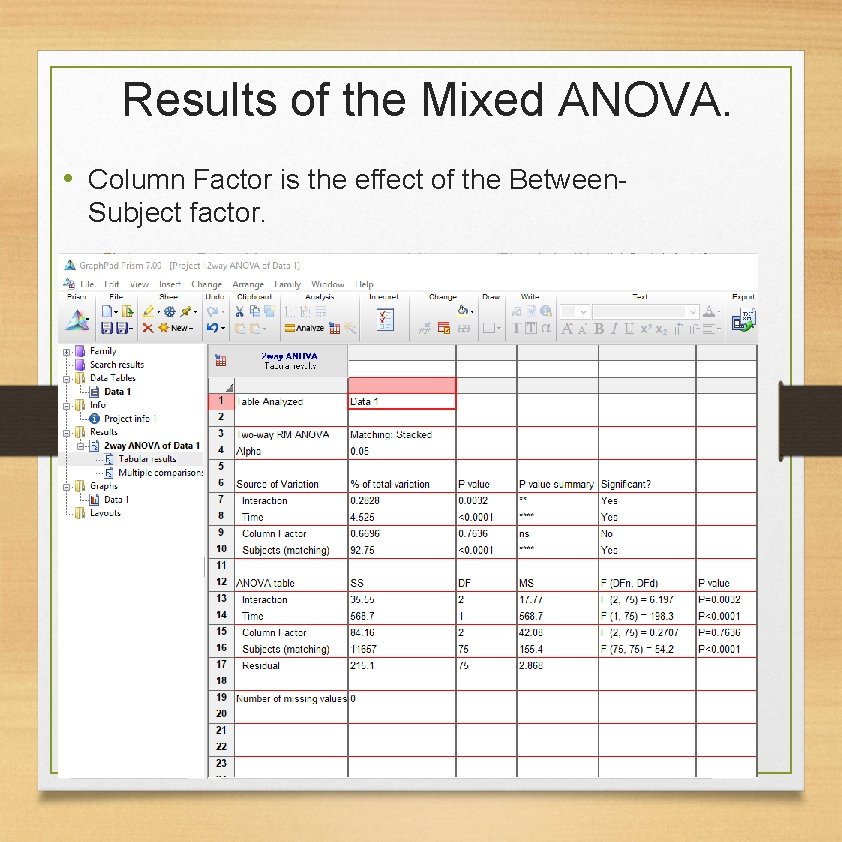
Results of the Mixed ANOVA. • Column Factor is the effect of the Between. Subject factor.

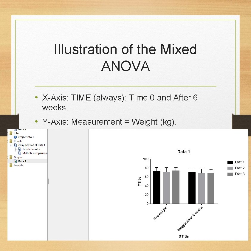
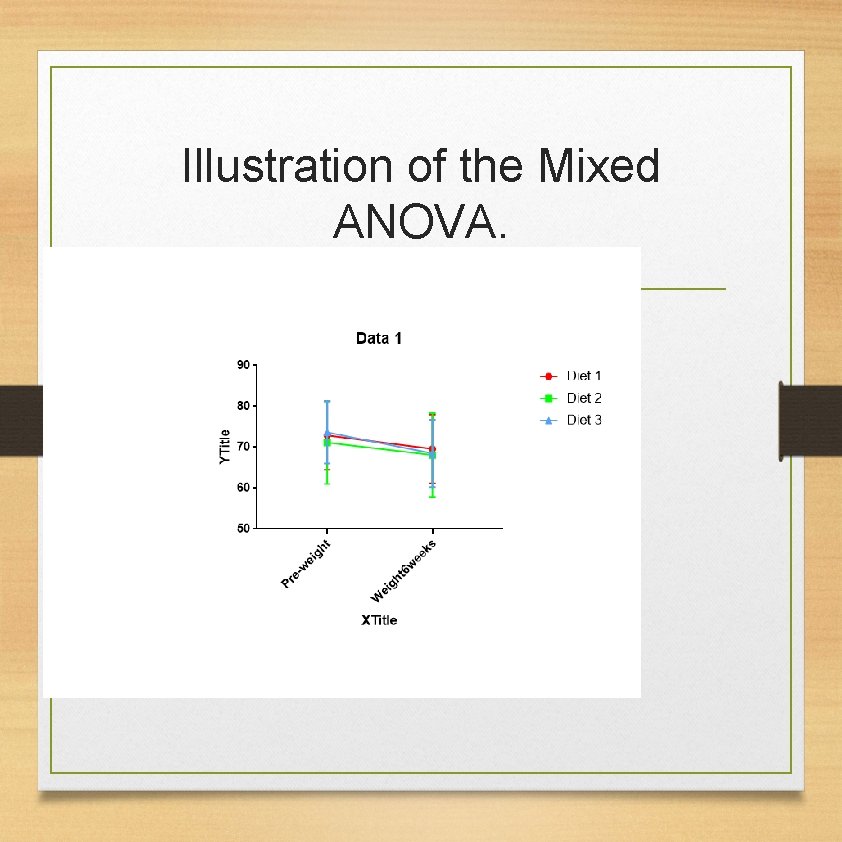
Illustration of the Mixed ANOVA • X-Axis: TIME (always): Time 0 and After 6 weeks. • Y-Axis: Measurement = Weight (kg). • Legend: Categorical Variable : Diet.

Illustration of the Mixed ANOVA.

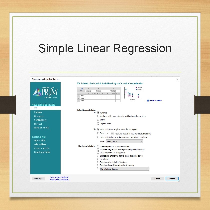
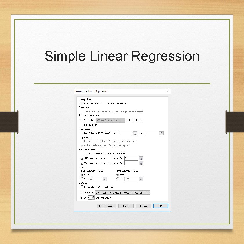
Simple Linear Regression • A simple linear regression is used when you want to predict a continuous Y by a continuous variable X. • Y is called the dependent variable. • X is called the independent variable or predictor.

Simple Linear Regression

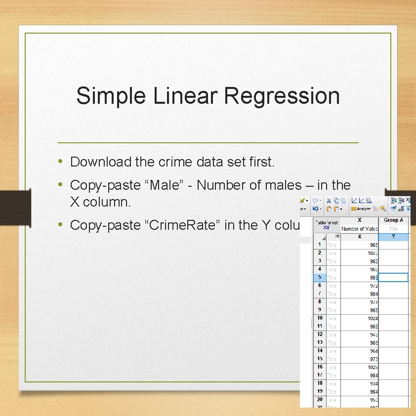
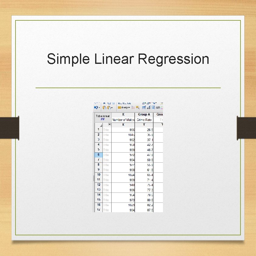
Simple Linear Regression • Download the crime data set first. • Copy-paste “Male” - Number of males – in the X column. • Copy-paste “Crime. Rate” in the Y column.

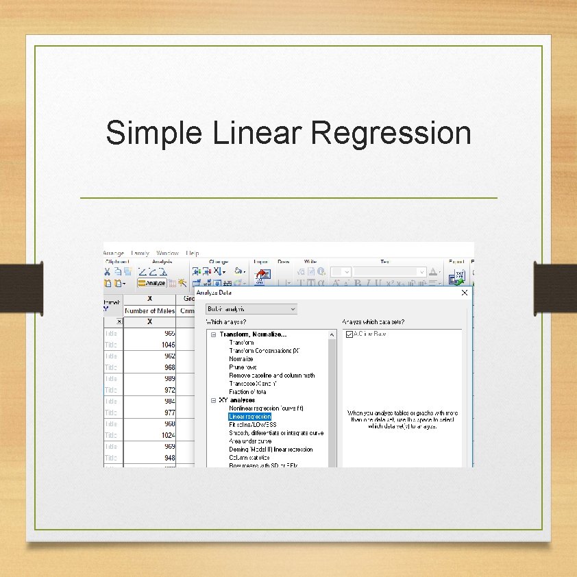
Simple Linear Regression

Simple Linear Regression

Simple Linear Regression

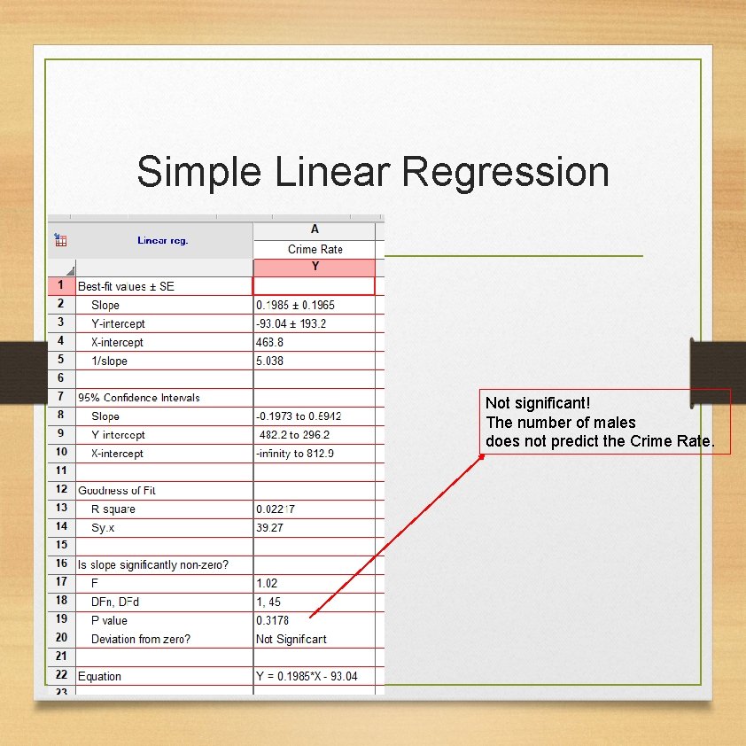
Simple Linear Regression Not significant! The number of males does not predict the Crime Rate.

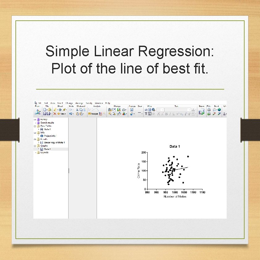
Simple Linear Regression: Plot of the line of best fit.

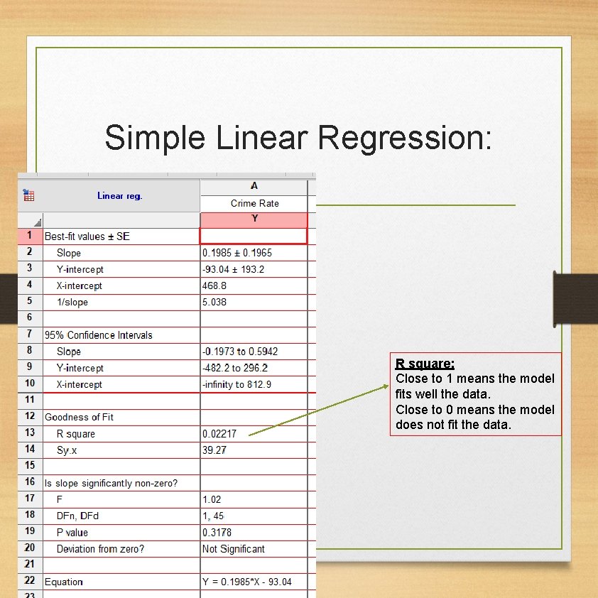
Simple Linear Regression: R square: Close to 1 means the model fits well the data. Close to 0 means the model does not fit the data.

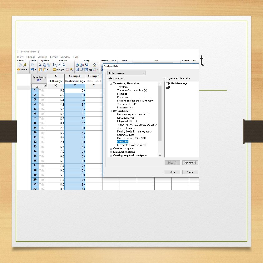
Simple Linear Regression • Try to do a simple linear regression to predict the birthweight (dependent variable Y) by the gestational age in the birthweight data set.

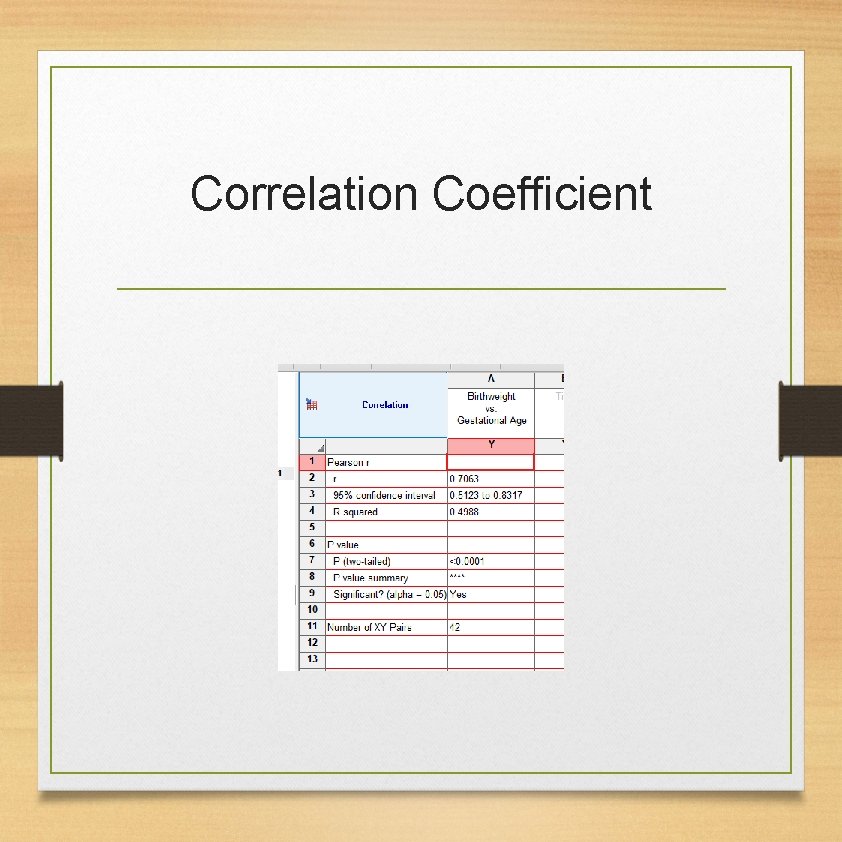
Correlation Coefficient

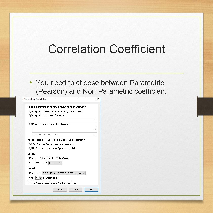
Correlation Coefficient • You need to choose between Parametric (Pearson) and Non-Parametric coefficient. How do you do that?

Correlation Coefficient