Graphing with Uncertainties Experimental data will contain uncertainties

Determine the acceleration… a Time (s) 0. 5 1 1. 5 2 2. 5

Raw Data with uncertainty Time (s) 0. 5 1 1. 5 2 2. 5

Transform data & uncertainties t (s) 0. 5 1 1. 5 2 2. 5

Add error bars Draw in line of BEST fit Draw in line of WORST

Line of best fit Line of worst fit Line of Best fit: Intercept =

Line of best fit: Intercept = -0. 29 cm Gradient = 1. 21 cms-2

Conclusion = State the relationship between the variables This statement shows § linear relationship

Slides: 14

Download presentation

Graphing with Uncertainties • Experimental data will contain uncertainties • These uncertainties now need to be considered when trying to determine the relationship between variables • Error bars are used to show the uncertainty in individual data points • Lines of best & worst fit are used to find the overall uncertainty in the relationship

Determine the acceleration… a Time (s) 0. 5 1 1. 5 2 2. 5 3 3. 5 4 d(cm) 0. 3 1. 15 1. 9 4. 5 7. 5 10. 2 14. 5 19 θ What are the Independent , dependent & control variables? Uncertainty in time values is ± 0. 05 s and d values are ± 10%

Raw Data with uncertainty Time (s) 0. 5 1 1. 5 2 2. 5 3 3. 5 4 ± (s) 0. 05 0. 05 d(cm) 0. 3 1. 15 1. 9 4. 5 7. 5 10. 2 14. 5 19 ± d(cm) 0. 03 0. 1 0. 2 0. 5 0. 8 1 1 2 Uncertainty in time values is ± 0. 05 s and d values are ± 10%

Raw Data with uncertainty Time (s) 0. 5 1 1. 5 2 2. 5 3 3. 5 4 ± (s) 0. 05 0. 05 d(cm) 0. 3 1. 15 or 1. 2 1. 9 4. 5 7. 5 10. 2 or 10 14. 5 or 15 19 ± d(cm) 0. 03 0. 1 0. 2 0. 5 0. 8 1 1 2 Uncertainty in time values is ± 0. 05 s and d values are ± 10%

d(cm) 30 25 20 15 10 5 0 0 -5 0. 5 1 1. 5 2 2. 5 3 3. 5 4 4. 5 Time (s) Not linear… guess relationship 5

Transform data & uncertainties t (s) 0. 5 1 1. 5 2 2. 5 3 3. 5 4 ± 0. 05 0. 05 ±% t 2(s 2) 10 0. 25 5 1. 0 3. 3 2. 5 4. 0 2 6. 3 1. 7 9. 0 1. 4 12. 3 16. 0 t + 0. 05 (s) ±% 20 10 6. 6 5 4 3. 4 2. 8 2. 6 ± 0. 05 0. 1 0. 2 0. 3 0. 4 d (cm) ± 0. 03 0. 1 1. 15 1. 2 0. 2 1. 9 0. 5 4. 5 0. 8 7. 5 1 10. 2 10 1 14. 5 15 2 19 19 d + 10% (cm)

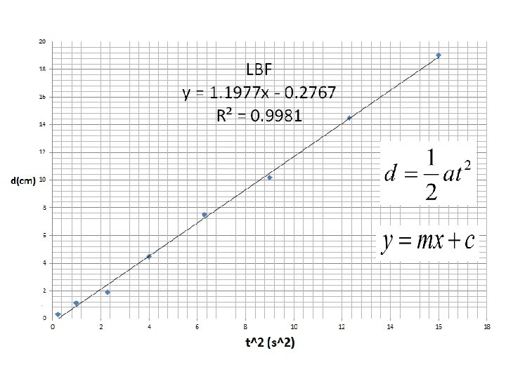
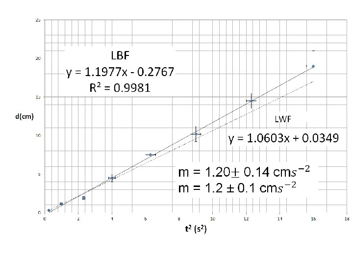
Add error bars Draw in line of BEST fit Draw in line of WORST fit This is some what arbitrary!

Line of best fit Line of worst fit Line of Best fit: Intercept = -0. 29 m Gradient = 1. 21 (3 sf) (from graphing calc) LABEL the lines Calculate gradients & record intercepts for BOTH lines Line of worst fit: Intercept = 0. 5 m Gradient = (16 -2)/(15 -2) = 1. 08

Line of best fit: Intercept = -0. 29 cm Gradient = 1. 21 cms-2 Line of worst fit: Intercept = 0. 5 cm Gradient = 1. 08 cms-2 Error uncertainties: Intercept = ( ) = ± 0. 8 cm Gradient = (1. 21 – 1. 08) = ± 0. 1 cms-2 State the relationship between the variables Round to 1 sf Conclusion Using: a = 2 x gradient = 2. 4 cms-2 Theoretical gradient = ? ? ? How does the experimental gradient value compares ? ? ? with theoretical value. Theoretical say it was 2. 8 cms-2 How does the experimental value compare?

Conclusion = State the relationship between the variables This statement shows § linear relationship between speed and time § error in the GRADIENT § error in the INTERCEPT § Try and include units (be careful about the y axis intercept units)