Graphing Radical Functions 3 You have seen the

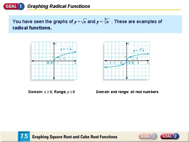
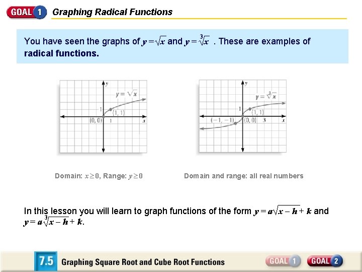
Graphing Radical Functions 3 You have seen the graphs of y = x and y = x. These are examples of radical functions. Domain: x ³ 0, Range: y ³ 0 Domain and range: all real numbers

Graphing Radical Functions 3 You have seen the graphs of y = x and y = x. These are examples of radical functions. Domain: x ³ 0, Range: y ³ 0 Domain and range: all real numbers In this lesson you will learn to graph functions of the form y = a x – h + k and 3 y = a x – h + k.

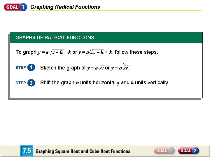
Graphing Radical Functions GRAPHS OF RADICAL FUNCTIONS 3 To graph y = a x – h + k or y = a x – h + k, follow these steps. 3 STEP 1 Sketch the graph of y = a x or y = a x. STEP 2 Shift the graph h units horizontally and k units vertically.

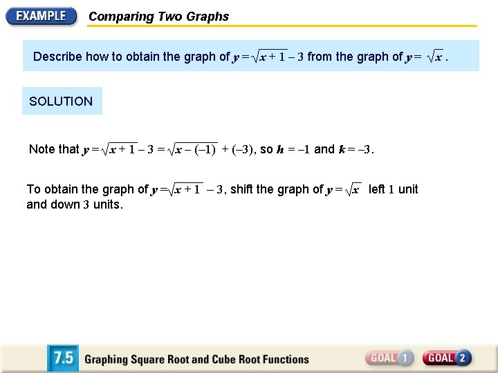
Comparing Two Graphs Describe how to obtain the graph of y = x + 1 – 3 from the graph of y = SOLUTION Note that y = x + 1 – 3 = x – (– 1) + (– 3), so h = – 1 and k = – 3. To obtain the graph of y = x + 1 – 3, shift the graph of y = x left 1 unit and down 3 units. x.

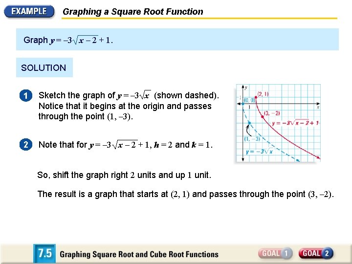
Graphing a Square Root Function Graph y = – 3 x – 2 + 1. SOLUTION 1 Sketch the graph of y = – 3 x (shown dashed). Notice that it begins at the origin and passes through the point (1, – 3). 2 Note that for y = – 3 x – 2 + 1, h = 2 and k = 1. So, shift the graph right 2 units and up 1 unit. The result is a graph that starts at (2, 1) and passes through the point (3, – 2).

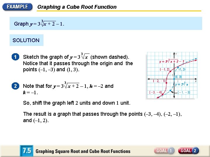
Graphing a Cube Root Function 3 Graph y = 3 x + 2 – 1. SOLUTION 3 1 Sketch the graph of y = 3 x (shown dashed). Notice that it passes through the origin and the points (– 1, – 3) and (1, 3). 2 Note that for y = 3 x + 2 – 1, h = – 2 and k = – 1. 3 So, shift the graph left 2 units and down 1 unit. The result is a graph that passes through the points (– 3, – 4), (– 2, – 1), and (– 1, 2).

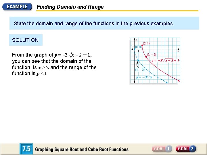
Finding Domain and Range State the domain and range of the functions in the previous examples. SOLUTION From the graph of y = – 3 x – 2 + 1, you can see that the domain of the function is x ³ 2 and the range of the function is y £ 1.

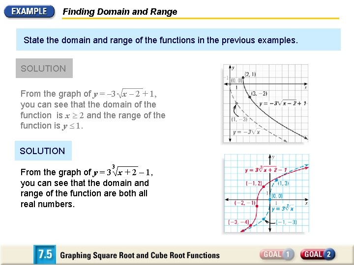
Finding Domain and Range State the domain and range of the functions in the previous examples. SOLUTION From the graph of y = – 3 x – 2 + 1, you can see that the domain of the function is x ³ 2 and the range of the function is y £ 1. SOLUTION 3 From the graph of y = 3 x + 2 – 1, you can see that the domain and range of the function are both all real numbers.

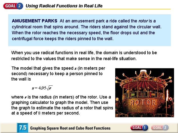
Using Radical Functions in Real Life AMUSEMENT PARKS At an amusement park a ride called the rotor is a cylindrical room that spins around. The riders stand against the circular wall. When the rotor reaches the necessary speed, the floor drops out and the centrifugal force keeps the riders pinned to the wall. When you use radical functions in real life, the domain is understood to be restricted to the values that make sense in the real-life situation. The model that gives the speed s (in meters per second) necessary to keep a person pinned to the wall is s = 4. 95 r where r is the radius (in meters) of the rotor. Use a graphing calculator to graph the model. Then use the graph to estimate the radius of a rotor that spins at a speed of 8 meters per second.

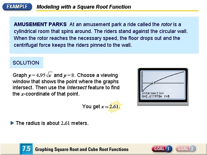
Modeling with a Square Root Function AMUSEMENT PARKS At an amusement park a ride called the rotor is a cylindrical room that spins around. The riders stand against the circular wall. When the rotor reaches the necessary speed, the floor drops out and the centrifugal force keeps the riders pinned to the wall. SOLUTION Graph y = 4. 95 x and y = 8. Choose a viewing window that shows the point where the graphs intersect. Then use the Intersect feature to find the x-coordinate of that point. You get x 2. 61. The radius is about 2. 61 meters.

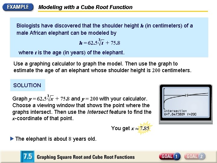
Modeling with a Cube Root Function Biologists have discovered that the shoulder height h (in centimeters) of a male African elephant can be modeled by 3 h = 62. 5 t + 75. 8 where t is the age (in years) of the elephant. Use a graphing calculator to graph the model. Then use the graph to estimate the age of an elephant whose shoulder height is 200 centimeters. SOLUTION 3 Graph y = 62. 5 x + 75. 8 and y = 200 with your calculator. Choose a viewing window that shows the point where the graphs intersect. Then use the Intersect feature to find the x-coordinate of that point. You get x 7. 85 The elephant is about 8 years old.