Graphical Sensitivity Analysis and Computer Solution Learning Objectives

Graphical Sensitivity Analysis and Computer Solution

Learning Objectives • Utilize graphical sensitivity analysis to answer what-if questions for the objective function coefficients and the right-Hand side values • Use a spreadsheet Solver and TORA to find optimal solution for an LP model • Understand the result of the spreadsheet Solver and TORA and interpret them

Sensitivity Analysis • Assumed that parameters are known with certainty • Parameters include the objective function coefficients, constraint quantity values, and constraint coefficients • Parameters are simply estimates • Effect of a parameter on the solution • Parameter changes and their effects on the model solution is known as sensitivity analysis

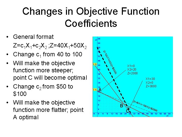
Changes in Objective Function Coefficients = X 2 50 + X 1 00 1 Z= X 1=0 X 2=20 Z=2000 $3 0 00 • General format Z=c 1 X 1+c 2 X 2 ; Z=40 X 1+50 X 2 • Change c 1 from 40 to 100 • Will make the objective function more steeper; point C will become optimal • Change c 2 from $50 to $100 • Will make the objective function more flatter; point A optimal X 1=30 X 2=0 Z=3000 A Z=4 0 X 1+ B C 100 X 2= $20 00

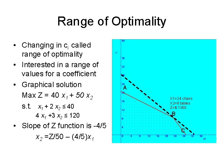
Range of Optimality • Changing in ci called range of optimality • Interested in a range of values for a coefficient • Graphical solution Max Z = 40 x 1 + 50 x 2 s. t. x 1 + 2 x 2 ≤ 40 4 x 1 +3 x 2 ≤ 120 • Slope of Z function is -4/5 x 2 =Z/50 – (4/5)x 1 A X 1=24 chairs X 2=8 tables Z=$ 1360 B C

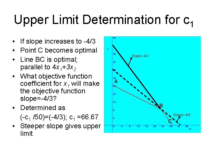
Upper Limit Determination for c 1 • If slope increases to -4/3 • Point C becomes optimal • Line BC is optimal; parallel to 4 x 1+3 x 2 • What objective function coefficient for x 1 will make the objective function slope=-4/3? • Determined as (-c 1 /50)=(-4/3); c 1 =66. 67 • Steeper slope gives upper limit Slope=-4/3 A B Slope=-4/5 C

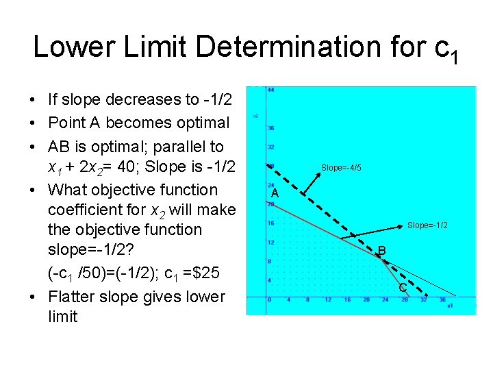
Lower Limit Determination for c 1 • If slope decreases to -1/2 • Point A becomes optimal • AB is optimal; parallel to x 1 + 2 x 2= 40; Slope is -1/2 • What objective function coefficient for x 2 will make the objective function slope=-1/2? (-c 1 /50)=(-1/2); c 1 =$25 • Flatter slope gives lower limit Slope=-4/5 A Slope=-1/2 B C

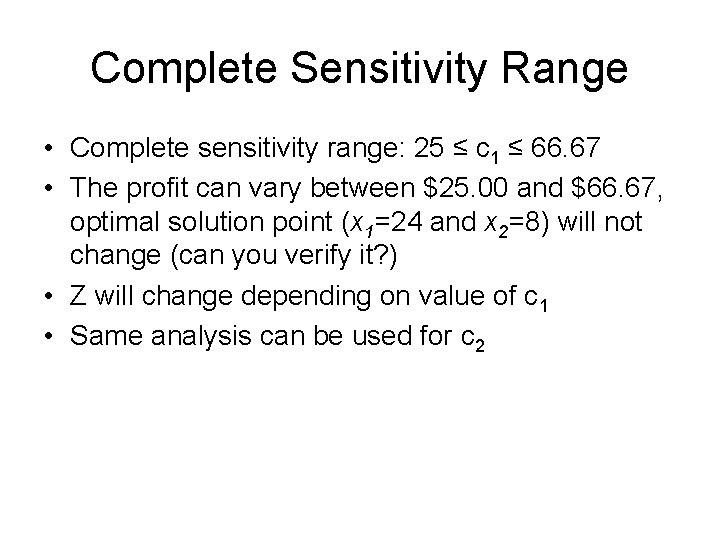
Complete Sensitivity Range • Complete sensitivity range: 25 ≤ c 1 ≤ 66. 67 • The profit can vary between $25. 00 and $66. 67, optimal solution point (x 1=24 and x 2=8) will not change (can you verify it? ) • Z will change depending on value of c 1 • Same analysis can be used for c 2

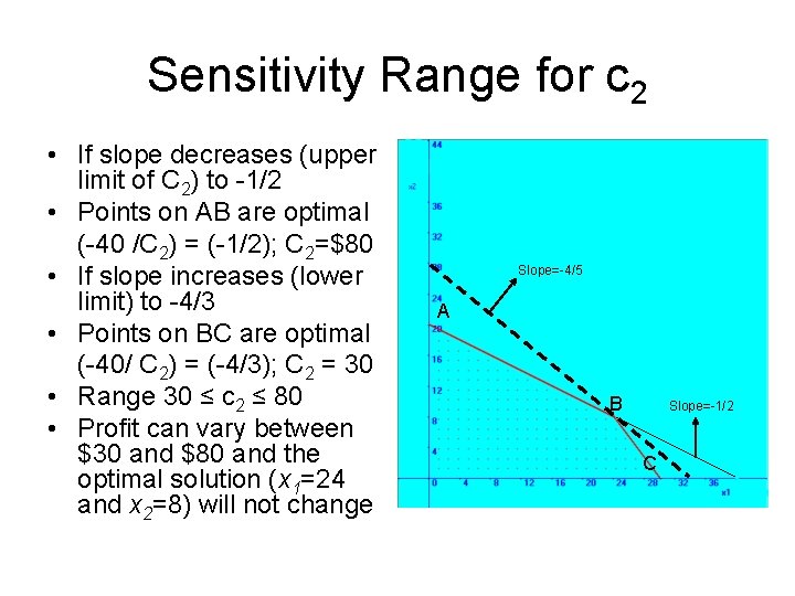
Sensitivity Range for c 2 • If slope decreases (upper limit of C 2) to -1/2 • Points on AB are optimal (-40 /C 2) = (-1/2); C 2=$80 • If slope increases (lower limit) to -4/3 • Points on BC are optimal (-40/ C 2) = (-4/3); C 2 = 30 • Range 30 ≤ c 2 ≤ 80 • Profit can vary between $30 and $80 and the optimal solution (x 1=24 and x 2=8) will not change Slope=-4/5 A B Slope=-1/2 C

Simultaneous Changes • Sensitivity range applies only if one coefficient is varied and the other one held constant • c 2: $30 ≤ profit for table ≤ $80, this is true only if c 1 remains constant • Simultaneous changes is overly complex and time-consuming using graphical analysis • Graphical analysis is a tedious way to perform sensitivity analysis

Feasibility Range • Sensitivity ranges for the right-hand side of constraints called feasibility range • Recall Max Z = $40 x 1 + 50 x 2 s. t. x 1 + 2 x 2 + s 1 = 40 (labor, hr) 4 x 1 + 3 x 2 + s 2 = 120 (wood, Ib) • Consider an increase in the availability of labor hours (from 40 to 60 hrs) without changing solution mix

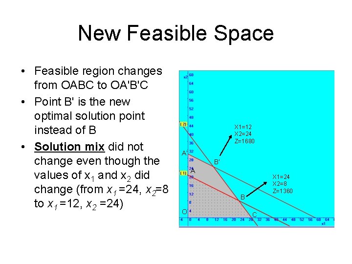
New Feasible Space • Feasible region changes from OABC to OA'B'C • Point B' is the new optimal solution point instead of B • Solution mix did not change even though the values of x 1 and x 2 did change (from x 1 =24, x 2=8 to x 1 =12, x 2 =24) X 1=12 X 2=24 Z=1680 A’ B’ A X 1=24 X 2=8 Z=1360 B O C

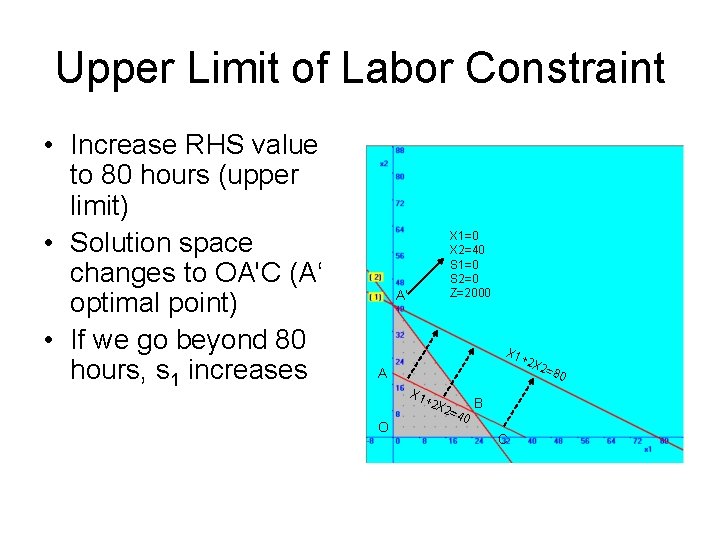
Upper Limit of Labor Constraint • Increase RHS value to 80 hours (upper limit) • Solution space changes to OA'C (A‘ optimal point) • If we go beyond 80 hours, s 1 increases X 1=0 X 2=40 S 1=0 S 2=0 Z=2000 A’ X 1+ 2 X 2 =80 A X 1 O +2 X 2=4 0 B C

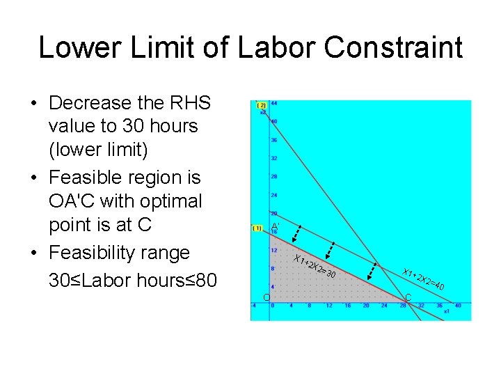
Lower Limit of Labor Constraint • Decrease the RHS value to 30 hours (lower limit) • Feasible region is OA'C with optimal point is at C • Feasibility range 30≤Labor hours≤ 80 A’ X 1 O +2 X 2=3 0 X 1+ 2 X 2= 40 C

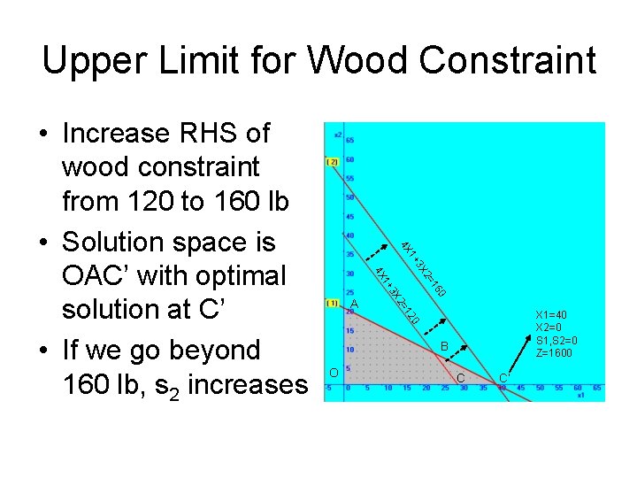
Upper Limit for Wood Constraint =1 X 2 +3 1 4 X 1 2= 3 X A 60 1+ 4 X X 1=40 X 2=0 S 1, S 2=0 Z=1600 20 • Increase RHS of wood constraint from 120 to 160 lb • Solution space is OAC’ with optimal solution at C’ • If we go beyond 160 lb, s 2 increases B O C C’

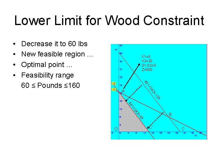
Lower Limit for Wood Constraint • • Decrease it to 60 lbs New feasible region. . . Optimal point … Feasibility range 60 ≤ Pounds ≤ 160 X 1=0 X 2=20 S 1, S 2=0 Z=800 +3 1 4 X 20 =1 X 2 A = X 2 +3 1 4 X 60 B O C’ C

Unit Worth a Resource • Feasibility range provides a single measure called unit worth of a shadow or resource price • Shows the rate of change in the optimal value as a result of making changes in the availability of a resource • Increased labor constraint from 40 to 80 hours, Z increased from $1360 to $2000 • Unit worth of labor constraint is $16 (2000 -1360)/(80 -40)=16 • Shows a 1 -hour change in labor constraint will change Z by $16

Dual Price • Represents the unit worth of a resource • Gives the contribution to the objective function resulting from a unit increase or decrease in the availability of a resource • Dual prices for labor and wood resources are $16/hour and $6/lb

RHS Sensitivity Analysis • Classify the constraint as either binding or nonbinding. – A binding constraint must pass through the optimum solution point. If it is not, it is nonbinding. – A binding constraint represents a scarce resource, whereas a nonbinding constraint represents an abundant resource. – An increase in a scarce resource can improve the value of the objective function

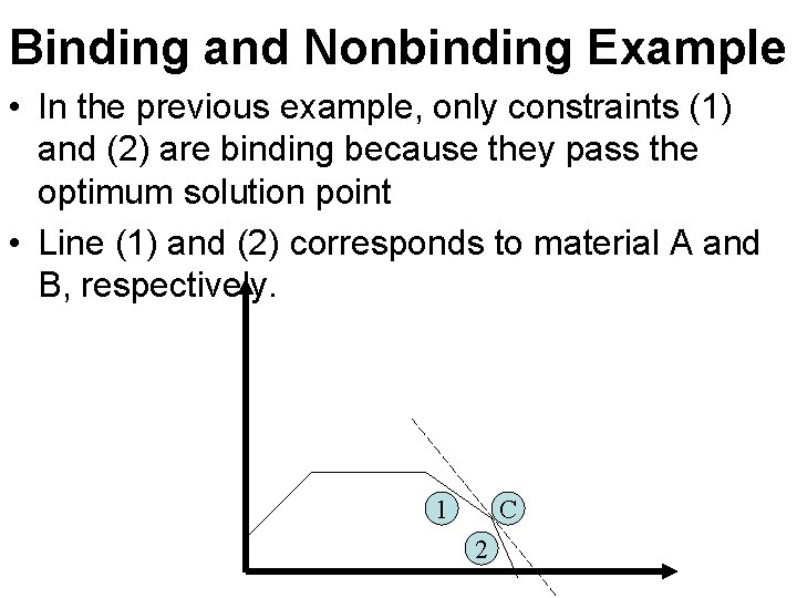
Binding and Nonbinding Example • In the previous example, only constraints (1) and (2) are binding because they pass the optimum solution point • Line (1) and (2) corresponds to material A and B, respectively. 1 C 2

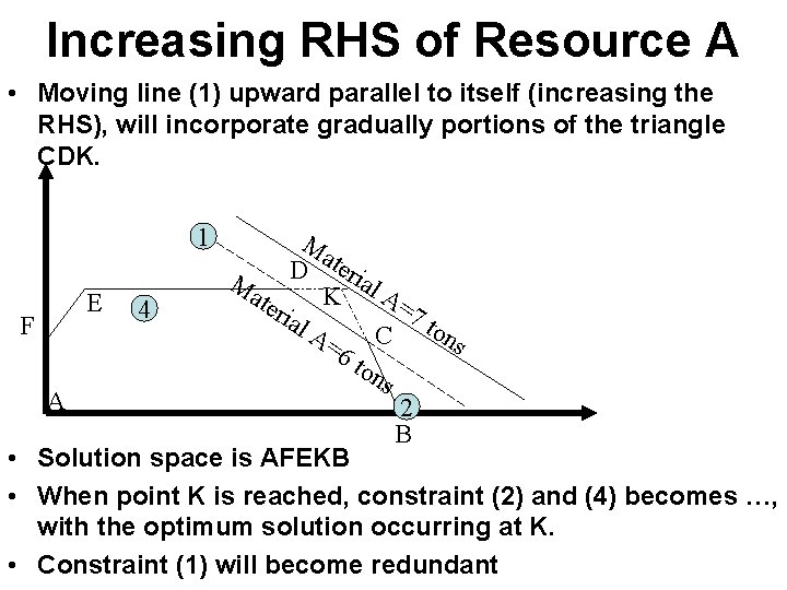
Increasing RHS of Resource A • Moving line (1) upward parallel to itself (increasing the RHS), will incorporate gradually portions of the triangle CDK. 1 Ma ter D ial Ma K A= ter E 4 7 t ial F A= C ons 6 t on s A 2 B • Solution space is AFEKB • When point K is reached, constraint (2) and (4) becomes …, with the optimum solution occurring at K. • Constraint (1) will become redundant

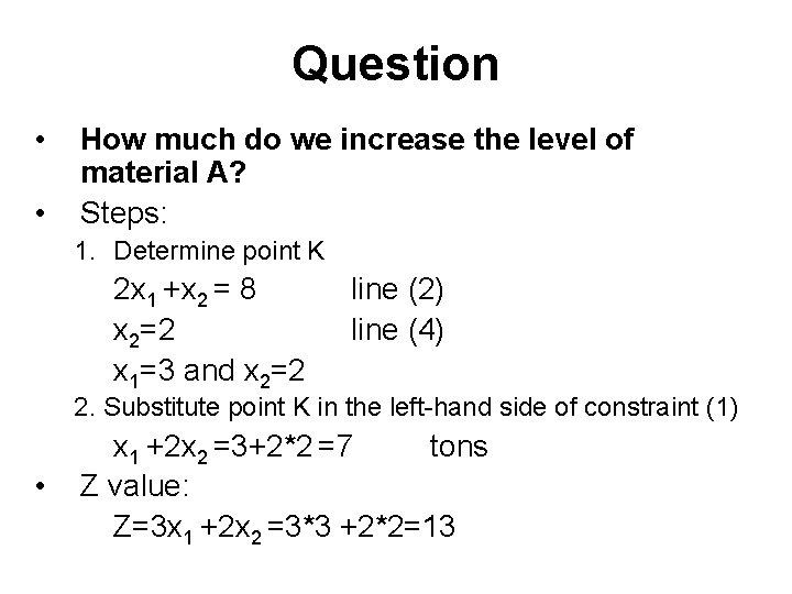
Question • • How much do we increase the level of material A? Steps: 1. Determine point K 2 x 1 +x 2 = 8 x 2=2 x 1=3 and x 2=2 line (2) line (4) 2. Substitute point K in the left-hand side of constraint (1) • x 1 +2 x 2 =3+2*2 =7 tons Z value: Z=3 x 1 +2 x 2 =3*3 +2*2=13

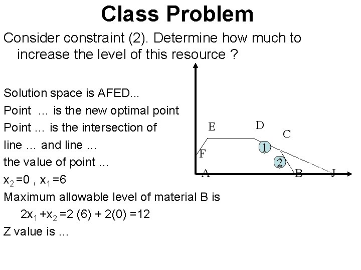
Class Problem Consider constraint (2). Determine how much to increase the level of this resource ? Solution space is AFED. . . Point … is the new optimal point E Point … is the intersection of line … and line … F the value of point … A x 2 =0 , x 1 =6 Maximum allowable level of material B is 2 x 1 +x 2 =2 (6) + 2(0) =12 Z value is … D C 1 2 B J

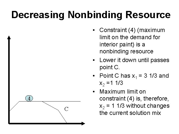
Decreasing Nonbinding Resource 4 C • Constraint (4) (maximum limit on the demand for interior paint) is a nonbinding resource • Lower it down until passes point C. • Point C has x 1 = 3 1/3 and x 2 =1 1/3 • Maximum limit on constraint (4) is, therefore, x 2 = 1 1/3 without changes the current solution mix

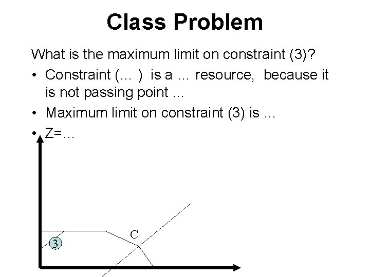
Class Problem What is the maximum limit on constraint (3)? • Constraint (… ) is a … resource, because it is not passing point … • Maximum limit on constraint (3) is … • Z=… 3 C

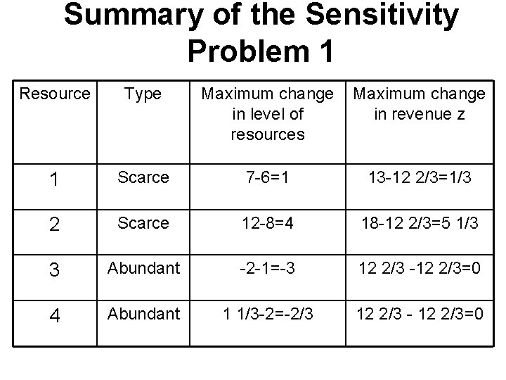
Summary of the Sensitivity Problem 1 Resource Type Maximum change in level of resources Maximum change in revenue z 1 Scarce 7 -6=1 13 -12 2/3=1/3 2 Scarce 12 -8=4 18 -12 2/3=5 1/3 3 Abundant -2 -1=-3 12 2/3 -12 2/3=0 4 Abundant 1 1/3 -2=-2/3 12 2/3 - 12 2/3=0

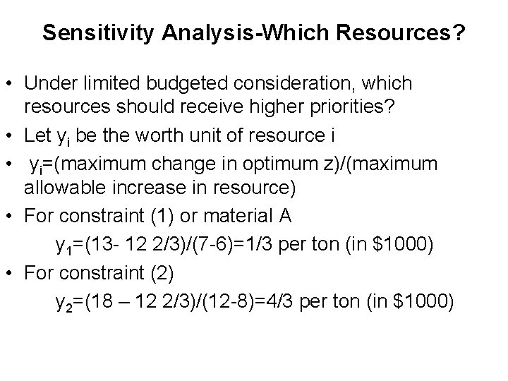
Sensitivity Analysis-Which Resources? • Under limited budgeted consideration, which resources should receive higher priorities? • Let yi be the worth unit of resource i • yi=(maximum change in optimum z)/(maximum allowable increase in resource) • For constraint (1) or material A y 1=(13 - 12 2/3)/(7 -6)=1/3 per ton (in $1000) • For constraint (2) y 2=(18 – 12 2/3)/(12 -8)=4/3 per ton (in $1000)

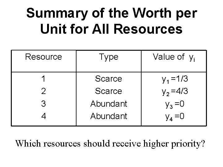
Summary of the Worth per Unit for All Resources Resource Type Value of yi 1 2 3 4 Scarce Abundant y 1 =1/3 y 2 =4/3 y 3 =0 y 4 =0 Which resources should receive higher priority?

Sensitivity Analysis-Sensitivity Problem 3 • How much change in the objective function coefficients? • Will change the slope of the objective function line • Will change the set of binding and nonbinding resources

Sensitivity Problem 3 Two Types of Situation 1. By how much can a coefficient be changed (increased or decreased) without changing the optimal solution point? 2. By how much can a coefficient be changed (increased or decreased) to reverse the status of a given resource?

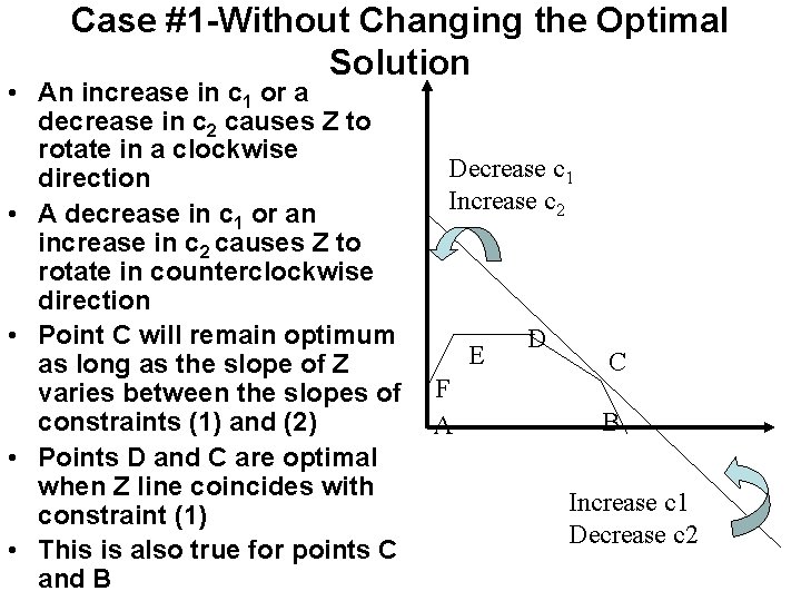
Case #1 -Without Changing the Optimal Solution • An increase in c 1 or a decrease in c 2 causes Z to rotate in a clockwise direction • A decrease in c 1 or an increase in c 2 causes Z to rotate in counterclockwise direction • Point C will remain optimum as long as the slope of Z varies between the slopes of constraints (1) and (2) • Points D and C are optimal when Z line coincides with constraint (1) • This is also true for points C and B Decrease c 1 Increase c 2 E F A D C B Increase c 1 Decrease c 2

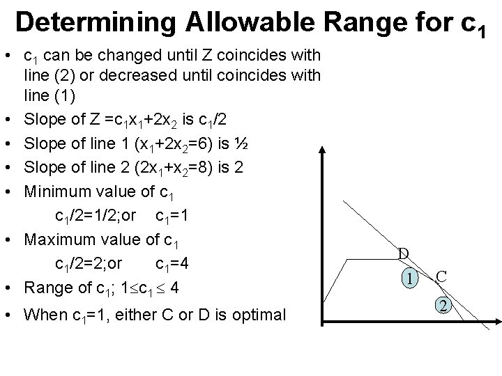
Determining Allowable Range for c 1 • c 1 can be changed until Z coincides with line (2) or decreased until coincides with line (1) • Slope of Z =c 1 x 1+2 x 2 is c 1/2 • Slope of line 1 (x 1+2 x 2=6) is ½ • Slope of line 2 (2 x 1+x 2=8) is 2 • Minimum value of c 1/2=1/2; or c 1=1 • Maximum value of c 1/2=2; or c 1=4 • Range of c 1; 1 c 1 4 • When c 1=1, either C or D is optimal D 1 C 2

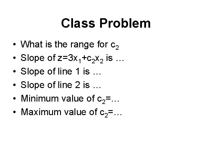
Class Problem • • • What is the range for c 2 Slope of z=3 x 1+c 2 x 2 is … Slope of line 1 is … Slope of line 2 is … Minimum value of c 2=… Maximum value of c 2=…

Computer Solution of the LP Model • Simplex method was used to solve LP Problems • Then computer was used to solve LP models using steps of simplex method • Computers popularized the LP technique • More than a dozen software that solve LP problems • Solve LP problems using Excel and TORA

Solution by Excel and TORA • Excel is more time-consuming than TORA • However the excel spreadsheet can be used as a template for programs • TORA is a menu-driven software • Not require user manual

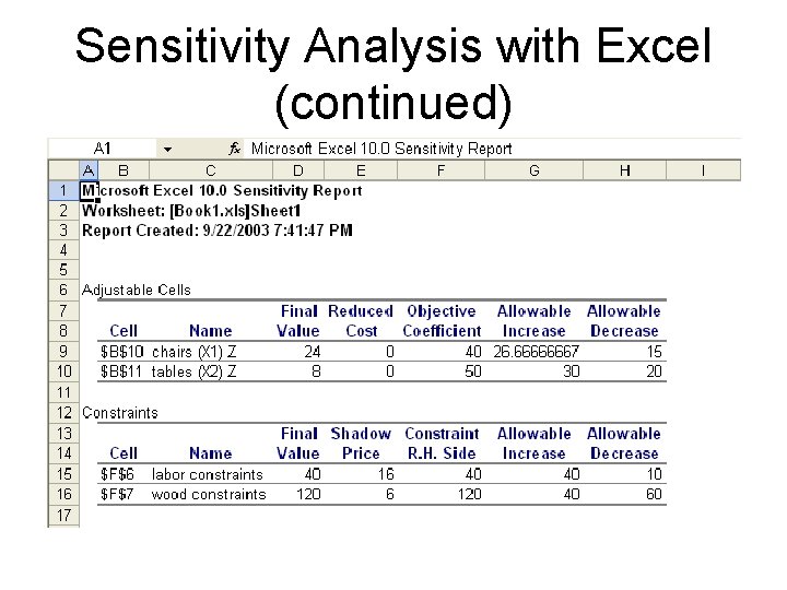
Sensitivity Analysis with Excel (continued)