Graphical Models II Dong Wang and Yang Feng

Graphical Models (II) Dong Wang and Yang Feng An introduction to Graphical Models – Michael Jordan CMU class 10708 – Eric Xing Probabilistic Graphical Models : Principles and Techiques – Daphne Koller

Outline • • Review of what we learned Start from simple models EM framework Approximate inference

What are graphical models? • Graphical models are probabilistic models represented in a graph form • Graphs represent (1) global structure (2) local dependency – Statistical independence can be read directly – The joint probability can be read directly – Inference can be conducted in a graphical way • Directed graphs (Bayesian networks) focuses on explicit dependency, undirected graphs (Markov fields) focuses on an implicit one. They are not equal, but in many cases can be converted from each other.

Graphical models and Neural network • They are different ways of balancing knowledge and experience • Some models belong to both, e. g. , stochastic NN and RBM • Graphical models are more generative, while NN is more used as discriminative

Supervised learning or unsupervised learning? • Graphical models can be either supervised or supervised • Targets are treated no difference from explaining variables • It is descriptive (generative), but descriptive for all variables – funny?

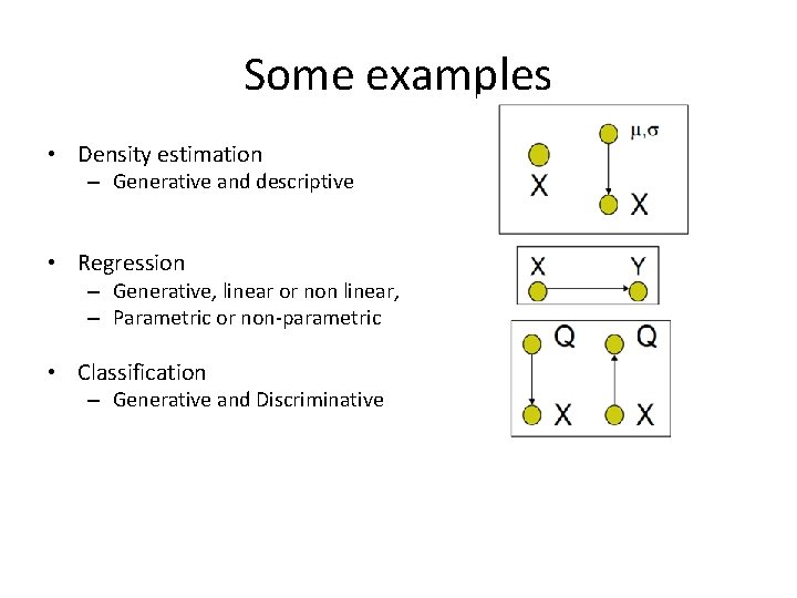
Some examples • Density estimation – Generative and descriptive • Regression – Generative, linear or non linear, – Parametric or non-parametric • Classification – Generative and Discriminative

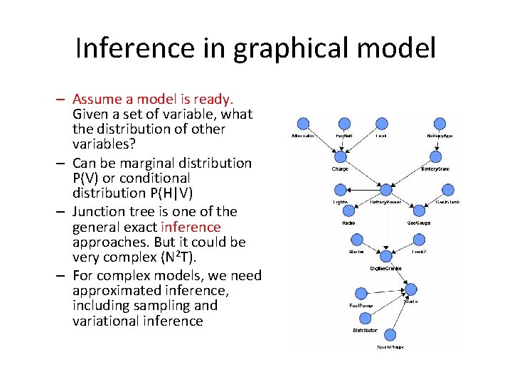
Inference in graphical model – Assume a model is ready. Given a set of variable, what the distribution of other variables? – Can be marginal distribution P(V) or conditional distribution P(H|V) – Junction tree is one of the general exact inference approaches. But it could be very complex (N 2 T). – For complex models, we need approximated inference, including sampling and variational inference

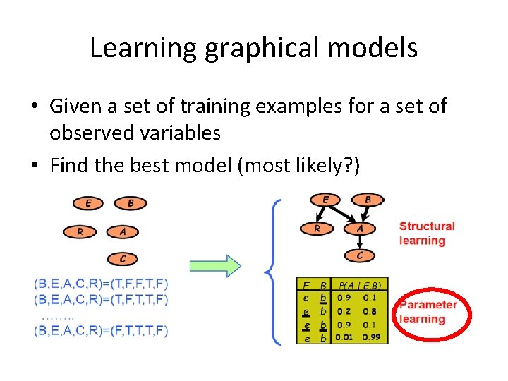
Learning graphical models • Given a set of training examples for a set of observed variables • Find the best model (most likely? )

Outline • • • Review of what we learned Start from simple models EM framework Inference Maximization

We start from some simple models • Gaussian mixture model (GMM) • Probabilistic PCA • Probabilistic linear discriminative analysis (PLDA) • Hidden Markov models (HMM) • Restrictive Boltzmann machines (RBM) • Conditional random filed (CRF) • Latent Dirichilet Allocation (LDA)

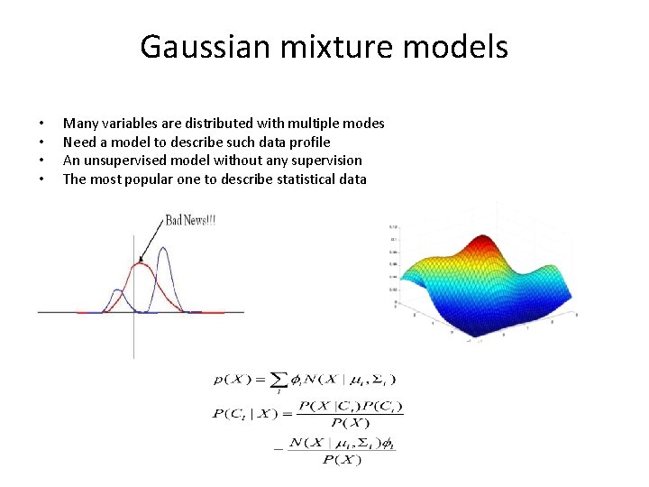
Gaussian mixture models • • Many variables are distributed with multiple modes Need a model to describe such data profile An unsupervised model without any supervision The most popular one to describe statistical data

GMM learning • The main difficulty of GMM – Hidden (latent) variables! • Solution – Make the hidden more explicit, in the way of probability estimation • An EM algorithm – E step: compute posteriors of unknown variables – M step: estimate model parameters with the estimated variables – Iterate until converge (? ) http: //www. juergenwiki. de/work/wiki/doku. php? id=public: gaussian_mixture_ models_em_algorithm_-_demo

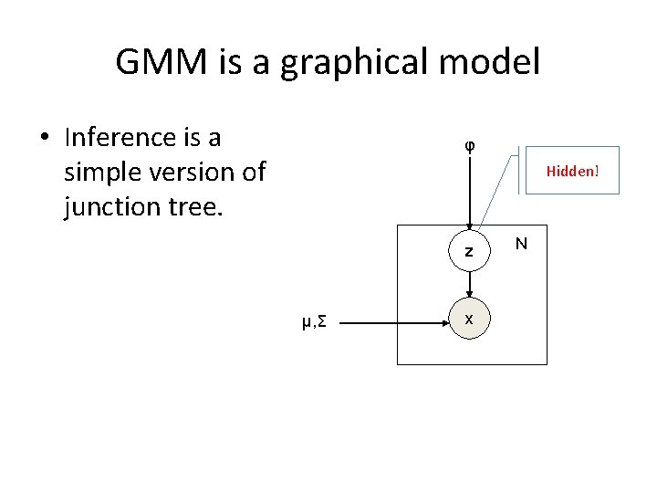
GMM is a graphical model • Inference is a simple version of junction tree. φ Hidden! z μ, Σ x N

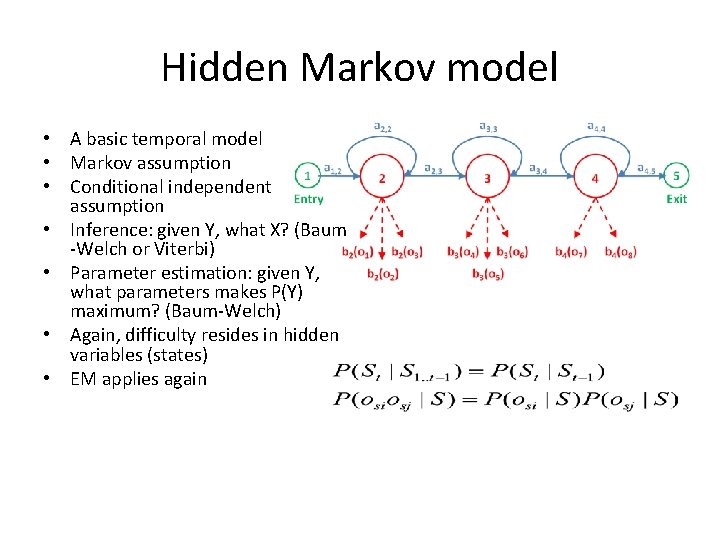
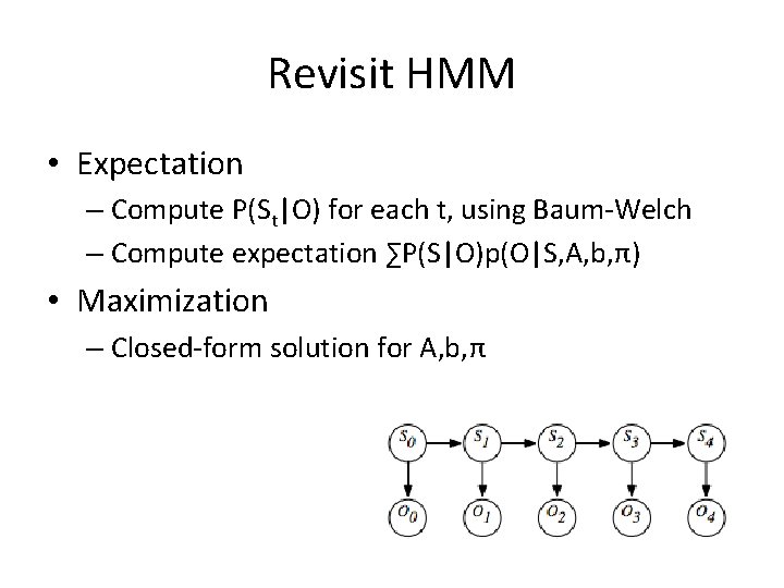
Hidden Markov model • A basic temporal model • Markov assumption • Conditional independent assumption • Inference: given Y, what X? (Baum -Welch or Viterbi) • Parameter estimation: given Y, what parameters makes P(Y) maximum? (Baum-Welch) • Again, difficulty resides in hidden variables (states) • EM applies again

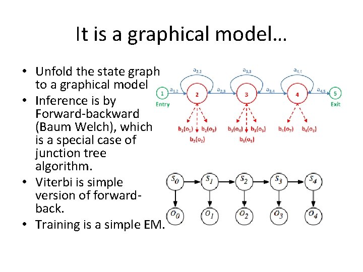
It is a graphical model… • Unfold the state graph to a graphical model • Inference is by Forward-backward (Baum Welch), which is a special case of junction tree algorithm. • Viterbi is simple version of forwardback. • Training is a simple EM.

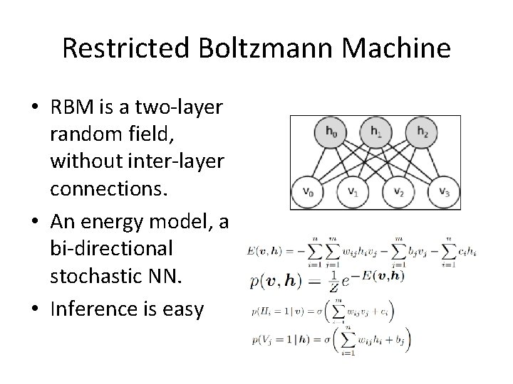
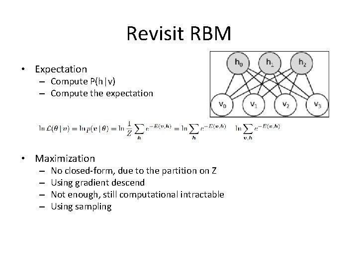
Restricted Boltzmann Machine • RBM is a two-layer random field, without inter-layer connections. • An energy model, a bi-directional stochastic NN. • Inference is easy

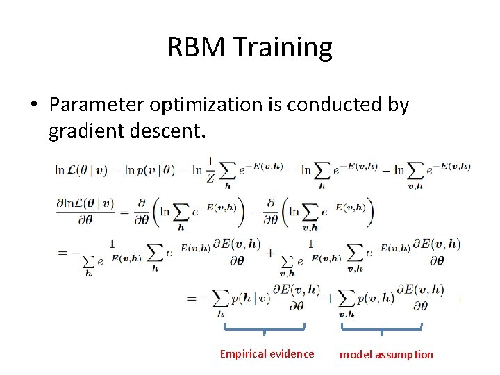
RBM Training • Parameter optimization is conducted by gradient descent. Empirical evidence model assumption

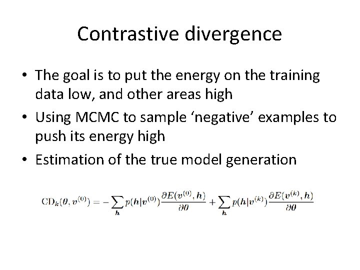
Contrastive divergence • The goal is to put the energy on the training data low, and other areas high • Using MCMC to sample ‘negative’ examples to push its energy high • Estimation of the true model generation

Outline • • Review of what we learned Start from simple models EM framework Approximate inference

It is time to think it more • We have seen diverse types of graphical models, and each seem has a particular training method. • We (may) have remembered numerous names: – K-mean, EM, CD, Viterbi, dynamic programing, junction tree, Baum-Welch, MCMC, SGD @$@%! • What are they? ?

Come back to difficulties • Some variables are random and hidden (latent) • Some dependences are complex • Some computations are intractable

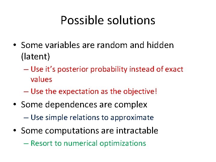
Possible solutions • Some variables are random and hidden (latent) – Use it’s posterior probability instead of exact values – Use the expectation as the objective! • Some dependences are complex – Use simple relations to approximate • Some computations are intractable – Resort to numerical optimizations

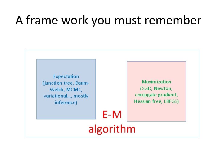
A frame work you must remember Expectation (junction tree, Baum. Welch, MCMC, variational…, mostly inference) Maximization (SGD, Newton, conjugate gradient, Hessian free, LBFGS) E-M algorithm

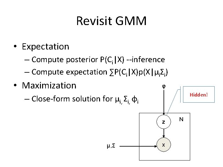
Revisit GMM • Expectation – Compute posterior P(Ci|X) --inference – Compute expectation ∑P(Ci|X)p(X|μiΣi) • Maximization φ Hidden! – Close-form solution for μi, Σi, φi z μ, Σ x N

Revisit HMM • Expectation – Compute P(St|O) for each t, using Baum-Welch – Compute expectation ∑P(S|O)p(O|S, A, b, π) • Maximization – Closed-form solution for A, b, π

Revisit RBM • Expectation – Compute P(h|v) – Compute the expectation • Maximization – – No closed-form, due to the partition on Z Using gradient descend Not enough, still computational intractable Using sampling

But things may be more complexed • So far, all the inference is simple • In complex graphical models, inference (posterior computation) could be intractable • We will discuss approximation inference method a bit late • Now let’s ask the question: will the EM procedure converge to what we want?

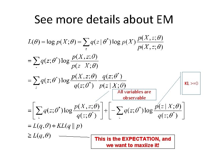
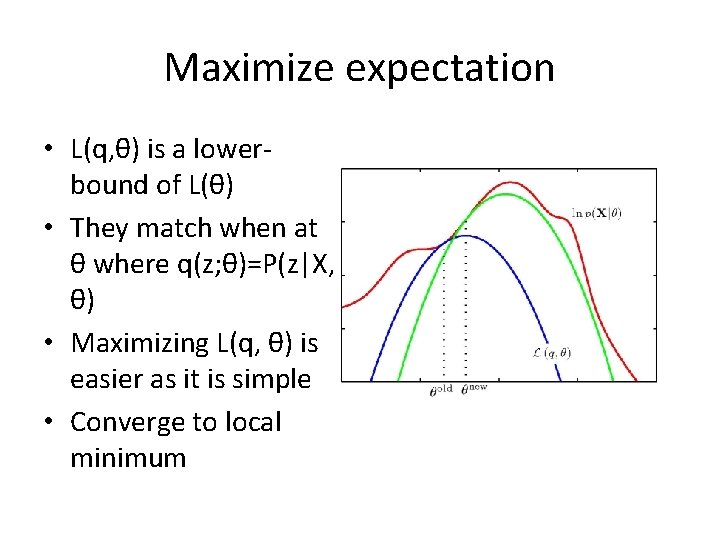
See more details about EM KL >=0 All variables are observable This is the EXPECTATION, and we want to maxiize it!

Maximize expectation • L(q, θ) is a lowerbound of L(θ) • They match when at θ where q(z; θ)=P(z|X, θ) • Maximizing L(q, θ) is easier as it is simple • Converge to local minimum

Outline • • Review of what we learned Start from simple models EM framework Approximate Inference

Intractable graphical models • Exact inference for some graphical models is tractable – Chain-like graphs – Tree-like graphs • Many graphical models do not have tractable exact inference – High dimensions. Complexity of message passing is O(TN 2) – Complex forms of posterior probabilities

Two approximated inference • Sampling approach – Use samples to represent posteriors or marginals • Variational approach – Use simpler functions to approximate posterios or marginals

Sampling approach • A graphical model is ‘generative’, and it can generate samples • Given a set of examples, we can compute statistics in a non-parametric or parametric way – Marginals, by ignoring uninterested variables – Conditionals, by categorizing the samples according to the values of the condtional varaibles • Directed graphical models can perform the sampling from parents to children • Undirected graphical models are not easy • Even the sampling is easy, it is usually highly inefficient, by wasting many samples.

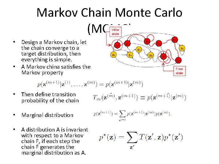
Markov Chain Monte Carlo (MCMC) • Design a Markov chain, let the chain converge to a target distribution, then everything is simple. • A Markov china satisfies the Markov property • Then define transition probability of the chain • Marginal distribution • A distribution A is invariant with respect to a Markov chain F, if each step the chain F generates the marginal distribution as A.

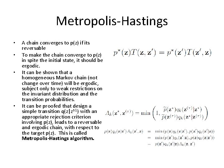
Metropolis-Hastings • • A chain converges to p(z) if its reversable To make the chain converge to p(z) in spite the initial state, it should be ergodic. It can be shown that a homogeneous Markov chain (not change over time) will be ergodic, subject only to weak restrictions on the invariant distribution and the transition probabilities. It can be proofed that design a simple transition q(z|zt-1) with an appropriate rejection criterion involving p(z), leads to a reversable and ergodic chain, with respect to the target p(z). This is called Metropolis-Hastings algorithm.

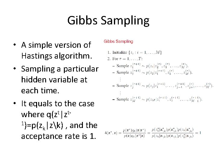
Gibbs Sampling • A simple version of Hastings algorithm. • Sampling a particular hidden variable at each time. • It equals to the case where q(zt|zt 1)=p(z |zk) , and the k acceptance rate is 1.

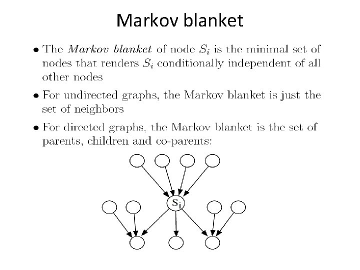
Determine the conditional • Need to check which variables the target variable depends on at each step • The set of variables a target variable depends on is called Markov blanket.

Markov blanket

Some problems of Gibbs sampling • It can take long time to converge • It is not simple to tell if it has converged • Successive samples are dependent. We can choose samples after every M sampling steps.

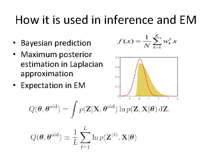
How it is used in inference and EM • Bayesian prediction • Maximum posterior estimation in Laplacian approximation • Expectation in EM

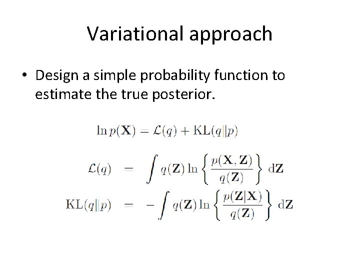
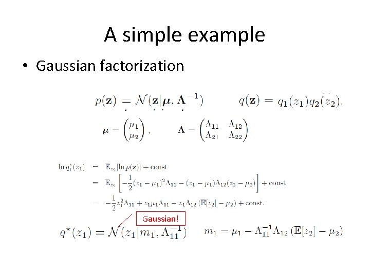
Variational approach • Design a simple probability function to estimate the true posterior.

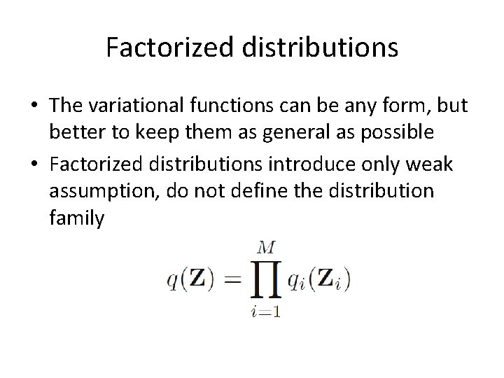
Factorized distributions • The variational functions can be any form, but better to keep them as general as possible • Factorized distributions introduce only weak assumption, do not define the distribution family

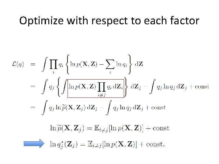
Optimize with respect to each factor

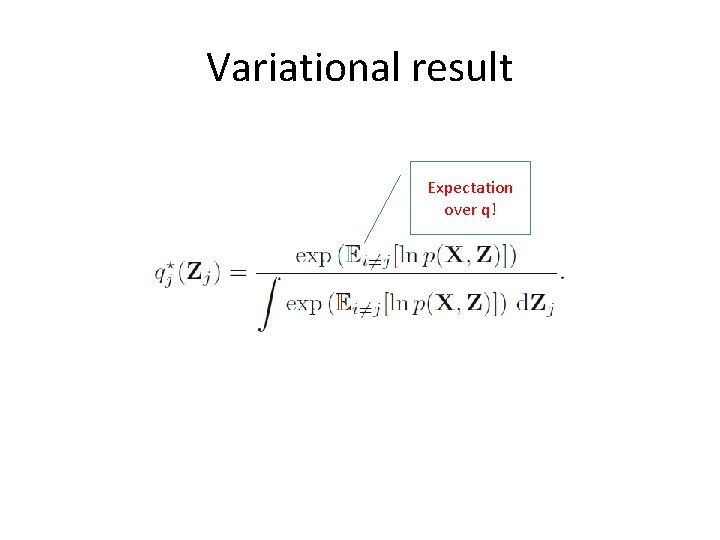
Variational result Expectation over q!

A simple example • Gaussian factorization Gaussian!

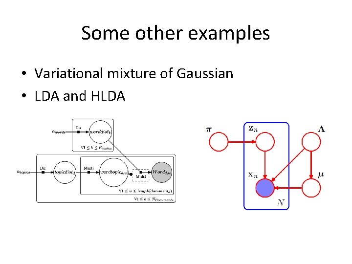
Some other examples • Variational mixture of Gaussian • LDA and HLDA

Cons and prons • Varational approach is generally fast than sampling, but still involves an iterative procedure • But it requires much design, most of time hard • We described a simpler variational approach that uses a deep NN to map variables to a space where the distribution is simple. But not much work how to infer variables in the new space – it is just for generation right now.

Wrap up • Graphical model is a structured model involves rich knowledge. It is a basic framework for complex inference. • Many models we used everyday belongs to graphical models. • A small set of graphical models can be inferred exactly with algorithms such as junction tree message passing • Most of the graphical models resort to approximate inference, particularly sampling and varitaional methods. • No matter how the inference is conducted, the EM is a general framework for model training.