Graph representation and traversal CISC 4080 Computer Algorithms

Graph: representation and traversal CISC 4080, Computer Algorithms CIS, Fordham Univ. Instructor: X. Zhang

Outline • Breath first search/traversal • review • Depth first search/traversal • … 2

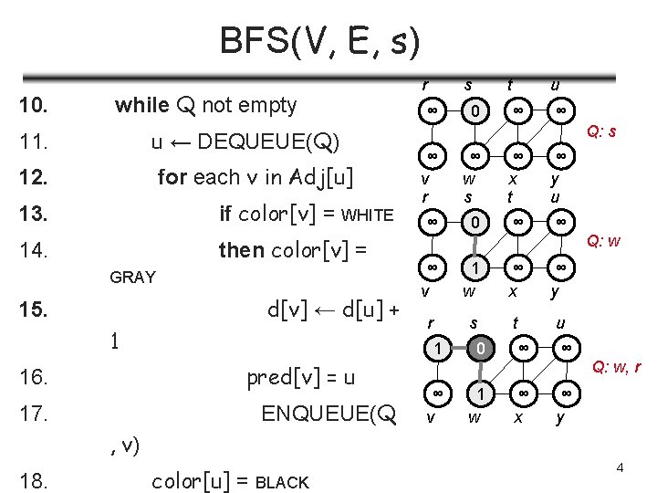
BFS(V, E, s) 1. for each u in V - {s} 2. do color[u] = WHITE 3. d[u] ← ∞ 4. pred[u] = 5. color[s] = NIL r s t u v r w s x t y u ∞ ∞ ∞ GRAY 6. d[s] ← 0 7. pred[s] = 8. Q = empty 9. ENQUEUE(Q, s) NIL ∞ v r ∞ w s ∞ x t ∞ y u ∞ 0 ∞ ∞ v w Q: s ∞ x ∞ y 3

BFS(V, E, s) 10. while Q not empty 11. u ← DEQUEUE(Q) 12. for each v in Adj[u] 13. if color[v] = WHITE 14. then color[v] = GRAY d[v] ← d[u] + 15. 1 pred[v] = u 16. 17. ENQUEUE(Q r s ∞ t 0 u ∞ ∞ Q: s ∞ v r ∞ w s ∞ x t ∞ y u ∞ 0 ∞ ∞ ∞ v 1 w ∞ x ∞ y r s t u 1 0 ∞ ∞ ∞ v 1 w ∞ x ∞ y Q: w, r , v) 18. color[u] = BLACK 4

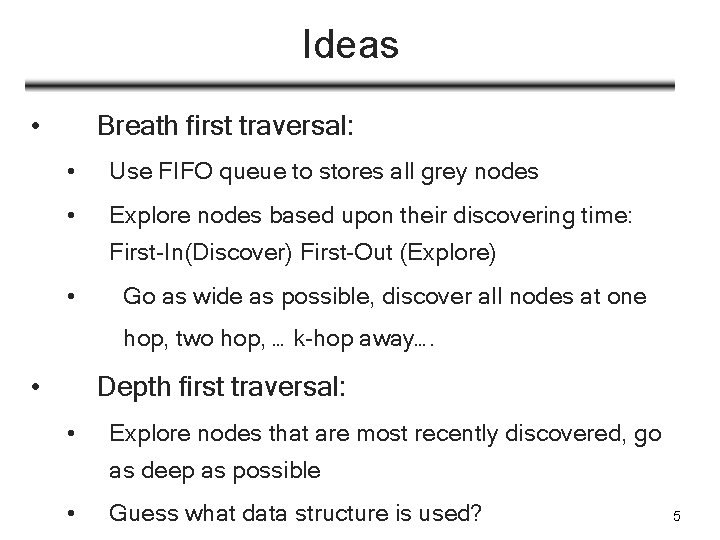
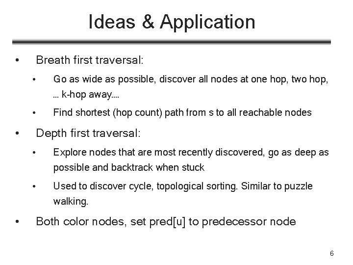
Ideas • Breath first traversal: • Use FIFO queue to stores all grey nodes • Explore nodes based upon their discovering time: First-In(Discover) First-Out (Explore) • Go as wide as possible, discover all nodes at one hop, two hop, … k-hop away…. • Depth first traversal: • Explore nodes that are most recently discovered, go as deep as possible • Guess what data structure is used? 5

Ideas & Application • Breath first traversal: • Go as wide as possible, discover all nodes at one hop, two hop, … k-hop away…. • • Find shortest (hop count) path from s to all reachable nodes Depth first traversal: • Explore nodes that are most recently discovered, go as deep as possible and backtrack when stuck • Used to discover cycle, topological sorting. Similar to puzzle walking. • Both color nodes, set pred[u] to predecessor node 6

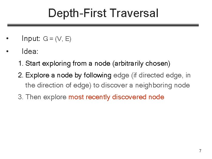
Depth-First Traversal • Input: G = (V, E) • Idea: 1. Start exploring from a node (arbitrarily chosen) 2. Explore a node by following edge (if directed edge, in the direction of edge) to discover a neighboring node 3. Then explore most recently discovered node 7

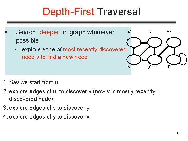
Depth-First Traversal • Search “deeper” in graph whenever possible u v w x y z • explore edge of most recently discovered node v to find a new node 1. Say we start from u 2. explore edges of u, to discover v (now v is mostly recently discovered node) 3. explore edges of v to discover y 4. explore edges of y to discover x 8

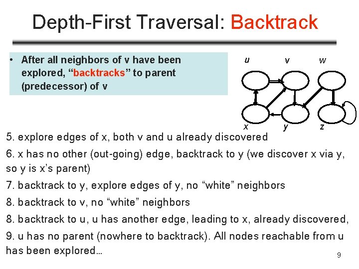
Depth-First Traversal: Backtrack • After all neighbors of v have been explored, “backtracks” to parent (predecessor) of v u v w x y z 5. explore edges of x, both v and u already discovered 6. x has no other (out-going) edge, backtrack to y (we discover x via y, so y is x’s parent) 7. backtrack to y, explore edges of y, no “white” neighbors 8. backtrack to v, no “white” neighbors 8. backtrack to u, u has another edge, leading to x, already discovered, 9. u has no parent (nowhere to backtrack). All nodes reachable from u has been explored… 9

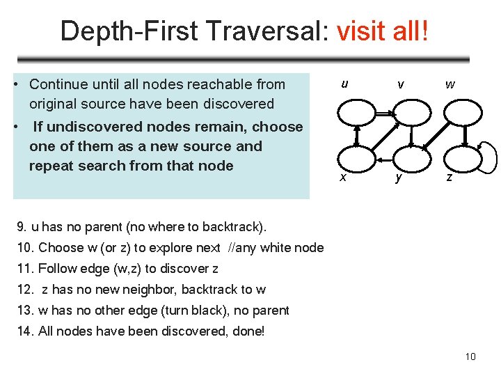
Depth-First Traversal: visit all! • Continue until all nodes reachable from original source have been discovered • If undiscovered nodes remain, choose one of them as a new source and repeat search from that node u v w x y z 9. u has no parent (no where to backtrack). 10. Choose w (or z) to explore next //any white node 11. Follow edge (w, z) to discover z 12. z has no new neighbor, backtrack to w 13. w has no other edge (turn black), no parent 14. All nodes have been discovered, done! 10

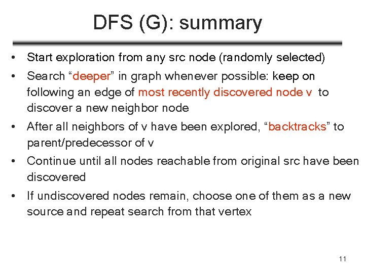
DFS (G): summary • Start exploration from any src node (randomly selected) • Search “deeper” in graph whenever possible: keep on following an edge of most recently discovered node v to discover a new neighbor node • After all neighbors of v have been explored, “backtracks” to parent/predecessor of v • Continue until all nodes reachable from original src have been discovered • If undiscovered nodes remain, choose one of them as a new source and repeat search from that vertex 11

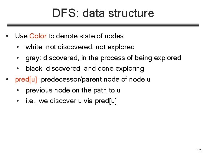
DFS: data structure • Use Color to denote state of nodes • white: not discovered, not explored • gray: discovered, in the process of being explored • black: discovered, and done exploring • pred[u]: predecessor/parent node of node u • previous node on the path to u • i. e. , we discover u via pred[u] 12

DFS Data Structures • d[u]– discovery time (when u turns gray) • f[u] – finish time (when u turns black) • during (d[u], f[u]), node u is grey • Instead of using wall-clock, we maintain: • virtual clock: an integer initialized to 0, incremented when something of interests happens, i. e. , nodes are discovered/finished 1 ≤ d[u] < f [u] 0 d[u] GRA Y f[u] time d[v] f[v] 13

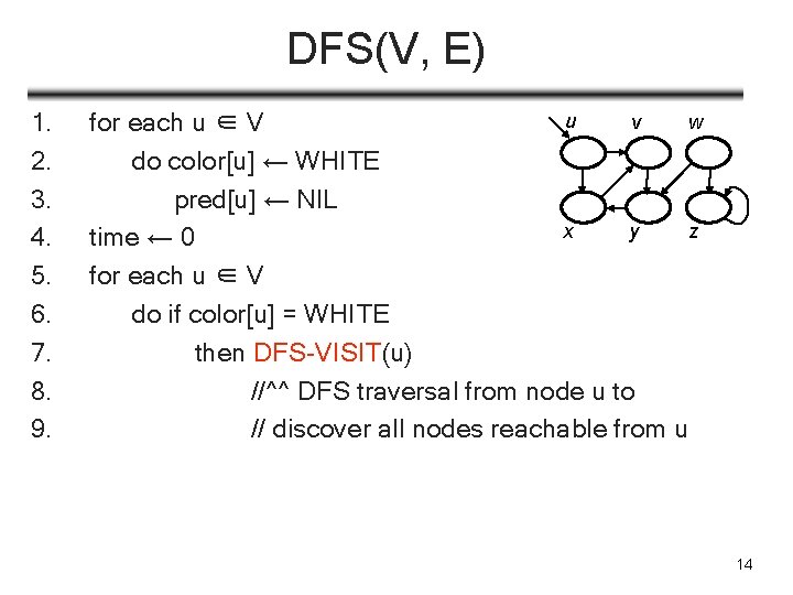
DFS(V, E) 1. 2. 3. 4. 5. 6. 7. 8. 9. u v w for each u ∈ V do color[u] ← WHITE pred[u] ← NIL x y z time ← 0 for each u ∈ V do if color[u] = WHITE then DFS-VISIT(u) //^^ DFS traversal from node u to // discover all nodes reachable from u 14

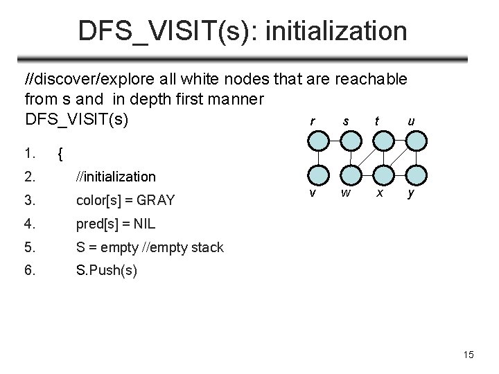
DFS_VISIT(s): initialization //discover/explore all white nodes that are reachable from s and in depth first manner DFS_VISIT(s) r s t u 1. { 2. //initialization 3. color[s] = GRAY 4. pred[s] = NIL 5. S = empty //empty stack 6. S. Push(s) v w x y 15

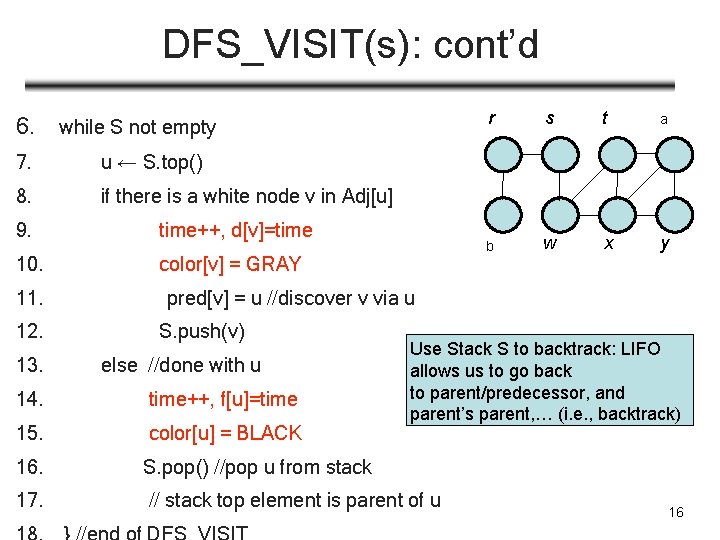
DFS_VISIT(s): cont’d 6. while S not empty 7. u ← S. top() 8. if there is a white node v in Adj[u] 9. time++, d[v]=time 10. color[v] = GRAY 11. 12. 13. r s t a u bv w x y pred[v] = u //discover v via u S. push(v) else //done with u Use Stack S to backtrack: LIFO allows us to go back to parent/predecessor, and parent’s parent, … (i. e. , backtrack) 14. time++, f[u]=time 15. color[u] = BLACK 16. S. pop() //pop u from stack 17. // stack top element is parent of u 16

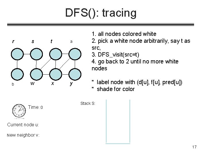
DFS(): tracing r s t ua v b w x y Time: 0 1. all nodes colored white 2. pick a white node arbitrarily, say t as src, 3. DFS_visit(src=t) 4. go back to 2 until no more white nodes * label node with (d[u], f[u], pred[u]) * shade for color Stack S: Current node u: New neighbor v: 17

DFS_VISIT(s) 1. { 2. //initialization 3. color[s] = GRAY 4. time++; d[s] = time 7. while S not empty 8. u ← S. top() 9. if there is a white node v in Adj[u] 10. S = empty //empty stack 11. 6. S. Push(s) 12. Push a node u into a stack: 5. start to explore u’s neighbors, neighbor’s neighbors Pop a node: done with it, go back to parent Like recursive calls! calling a function => push to call stack return from a function call => pop call stack 13. 14. time++, d[v]=time color[v] = GRAY pred[v] = u //discover v via u S. push(v) else //done with u 15. time++, f[u]=time 16. color[u] = BLACK 17. S. pop() //pop u from stack 18. } //end of DFS_VISIT 18

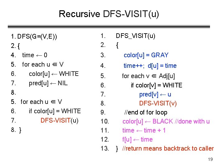
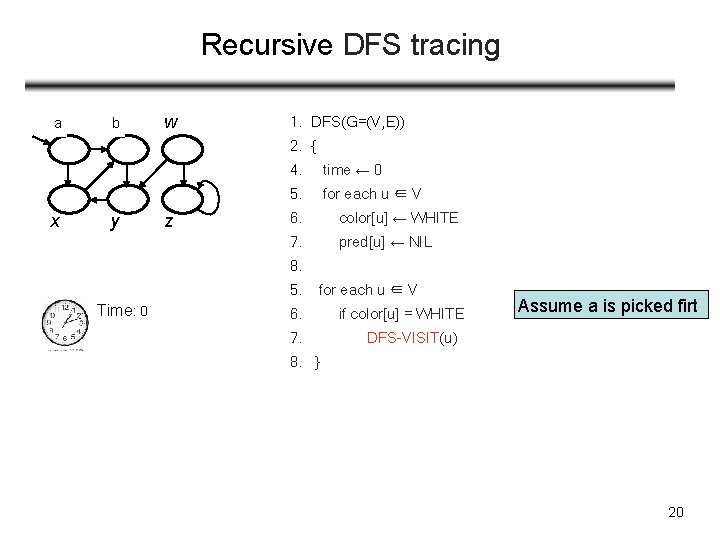
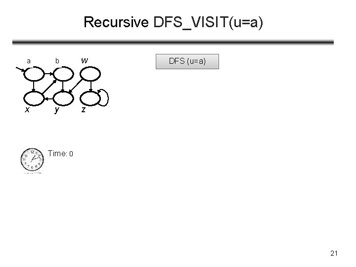
Recursive DFS-VISIT(u) 1. DFS(G=(V, E)) 2. { 4. time ← 0 5. for each u ∈ V 6. color[u] ← WHITE 7. pred[u] ← NIL 8. 5. for each u ∈ V 6. if color[u] = WHITE 7. DFS-VISIT(u) 8. } 1. 2. DFS_VISIT(u) { 3. color[u] = GRAY 4. time++; d[u] = time 5. 6. 7. 8. 9. 10. 11. 12. 13. for each v ∈ Adj[u] if color[v] = WHITE pred[v] ← u DFS-VISIT(v) //end of for loop color[u] ← BLACK //done with u time ← time + 1 f[u] ← time } //return means backtrack to caller 19

Recursive DFS tracing ua b v w 1. DFS(G=(V, E)) 2. { x y z 4. time ← 0 5. for each u ∈ V 6. color[u] ← WHITE 7. pred[u] ← NIL 8. 5. Time: 0 for each u ∈ V 6. 7. if color[u] = WHITE Assume a is picked firt DFS-VISIT(u) 8. } 20

Recursive DFS_VISIT(u=a) ua b v w x y z DFS (u=a) Time: 0 21

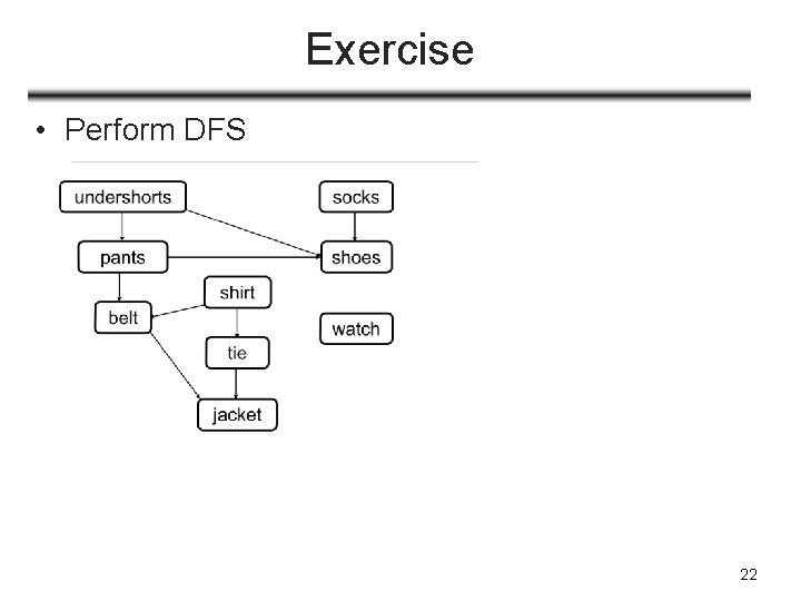
Exercise • Perform DFS 22

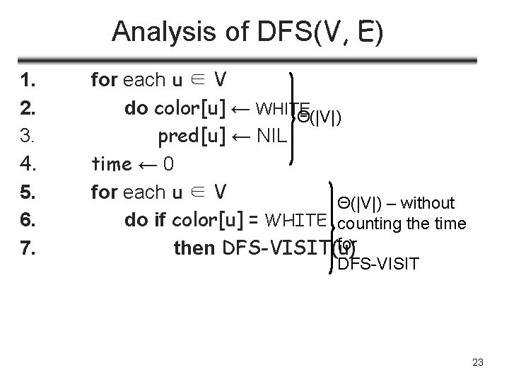
Analysis of DFS(V, E) 1. 2. 3. 4. 5. 6. 7. for each u ∈ V do color[u] ← WHITE Θ(|V|) pred[u] ← NIL time ← 0 for each u ∈ V Θ(|V|) – without do if color[u] = WHITE counting the time for then DFS-VISIT(u) DFS-VISIT 23

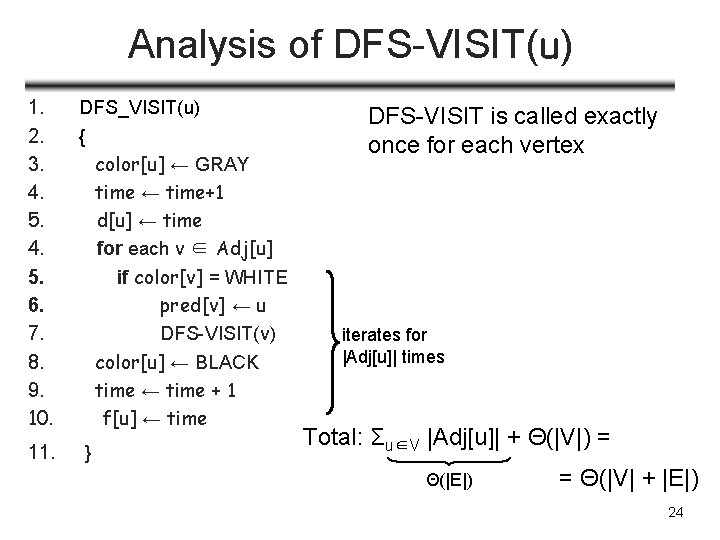
Analysis of DFS-VISIT(u) 1. 2. 3. 4. 5. 6. 7. 8. 9. 10. DFS_VISIT(u) { color[u] ← GRAY time ← time+1 d[u] ← time for each v ∈ Adj[u] if color[v] = WHITE pred[v] ← u DFS-VISIT(v) color[u] ← BLACK time ← time + 1 f[u] ← time 11. } DFS-VISIT is called exactly once for each vertex iterates for |Adj[u]| times Total: Σu∈V |Adj[u]| + Θ(|V|) = Θ(|E|) = Θ(|V| + |E|) 24

Next • DFS Forest • Different edges: tree edge, back edge, … • Application of DFS • cycle detection • topological sorting 25

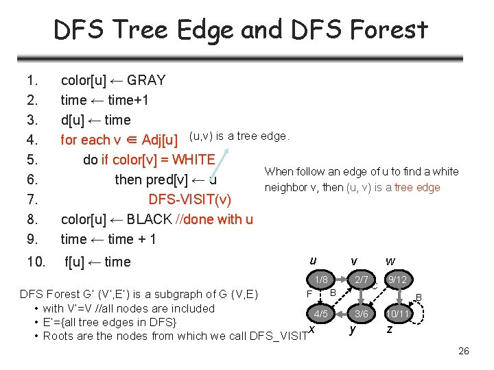
DFS Tree Edge and DFS Forest 1. 2. 3. 4. 5. 6. 7. 8. 9. color[u] ← GRAY time ← time+1 d[u] ← time for each v ∈ Adj[u] (u, v) is a tree edge. do if color[v] = WHITE When follow an edge of u to find a white then pred[v] ← u neighbor v, then (u, v) is a tree edge DFS-VISIT(v) color[u] ← BLACK //done with u time ← time + 1 10. f[u] ← time u 1/8 B F DFS Forest G’ (V’, E’) is a subgraph of G (V, E) • with V’=V //all nodes are included 4/5 • E’={all tree edges in DFS} x • Roots are the nodes from which we call DFS_VISIT v 2/7 w C 9/12 B 3/6 y 10/11 z 26

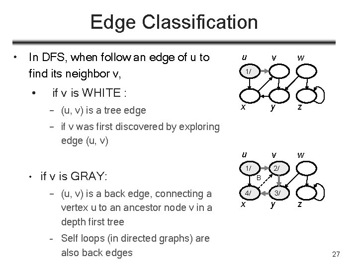
Edge Classification • In DFS, when follow an edge of u to find its neighbor v, • u v w x y z u v w 1/ if v is WHITE : – (u, v) is a tree edge – if v was first discovered by exploring edge (u, v) • if v is GRAY: – (u, v) is a back edge, connecting a vertex u to an ancestor node v in a depth first tree – Self loops (in directed graphs) are also back edges 1/ 2/ B 4/ x 3/ y z 27

Edge Classification • if v is BLACK, and d[u] < d[v]: – (u, v) is forward edge, non-tree edge that connects a vertex u to a descendant v in a depth first tree • u v 1/ w 2/7 B F 4/5 3/6 x y z u v w if v is BLACK and d[u] > d[v]: – (u, v) is cross edge – Can go between vertices in same depth-first tree (as long as there is no ancestor / descendant relation) or between different depth-first trees 1/8 2/7 B F 4/5 x 9/ C 3/6 y z – e. g. , (w, y) in example 28

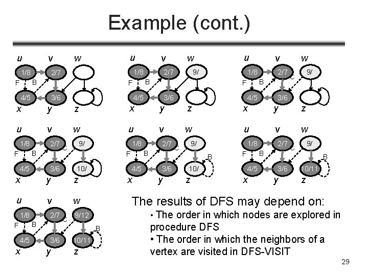
Example (cont. ) u v 1/8 u w 1/8 2/7 B F v 2/7 v 1/8 3/6 2/7 B F 4/5 3/6 9/ B F 4/5 u w 4/5 w 9/ C 3/6 x y z u v w 1/8 2/7 B F 4/5 3/6 10/ y z u v w 2/7 B F 4/5 x C 4/5 x y z 1/8 B 3/6 y 10/ z 2/7 B F 4/5 x 9/ C B 3/6 y 10/11 z • The order in which nodes are explored in 9/12 10/11 9/ C The results of DFS may depend on: B 3/6 2/7 B F x 1/8 9/ C procedure DFS • The order in which the neighbors of a vertex are visited in DFS-VISIT 29

Predecessor and Descendant u • u = pred[v] �DFS-VISIT(v) was called 1/ during a search of u’s adjacency list • u is “direct” predecessor of v • v is “direct” descendant of u • v w 2/ 3/ x y z Vertex v is a descendant of vertex u in depth first forest �v is discovered while u is gray • if we follow predecessor pointers(a back pointer to predecessor node) from v, we will reach u 30

Other Properties of DFS Corollary u Vertex v is a descendant of u �d[u] < d[v] < f[u] i. e. , v is discovered after u is discovered, v is finished before u is finished 1/8 2/7 B F 4/5 C 9/12 B 3/6 10/11 v Verify this using the example 31

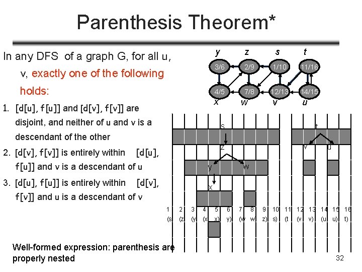
Parenthesis Theorem* y z v, exactly one of the following 3/6 2/9 1/10 11/16 holds: 4/5 7/8 12/13 14/15 v u In any DFS of a graph G, for all u, x 1. [d[u], f[u]] and [d[v], f[v]] are disjoint, and neither of u and v is a s w t s t descendant of the other 2. [d[v], f[v]] is entirely within f[u]] and v is a descendant of u 3. [d[u], f[u]] is entirely within v z [d[u], w y [d[v], u x f[v]] and u is a descendant of v 1 2 3 4 5 6 7 (s (z (y (x x) y) (w w) z) s) Well-formed expression: parenthesis are properly nested 8 9 10 11 12 13 14 15 16 (t (v v) (u u) 32 t)

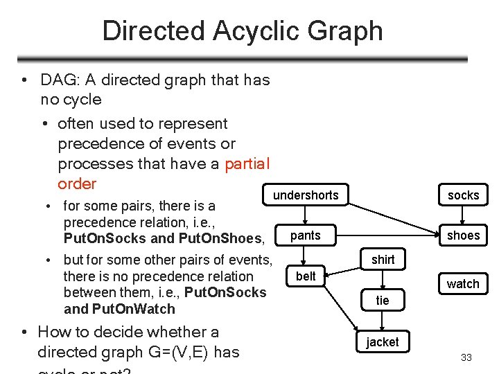
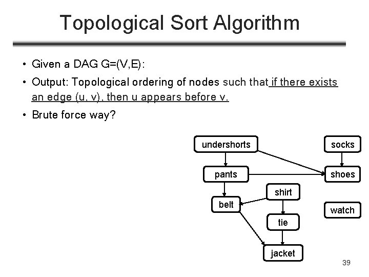
Directed Acyclic Graph • DAG: A directed graph that has no cycle • often used to represent precedence of events or processes that have a partial order undershorts socks pants shoes • for some pairs, there is a precedence relation, i. e. , Put. On. Socks and Put. On. Shoes, • but for some other pairs of events, there is no precedence relation between them, i. e. , Put. On. Socks and Put. On. Watch • How to decide whether a directed graph G=(V, E) has shirt belt watch tie jacket 33

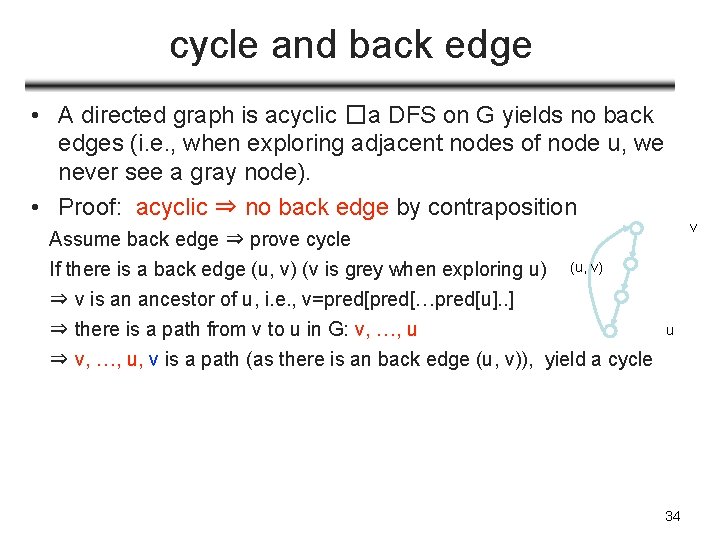
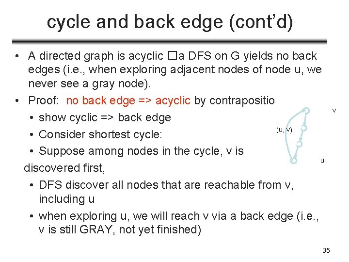
cycle and back edge • A directed graph is acyclic �a DFS on G yields no back edges (i. e. , when exploring adjacent nodes of node u, we never see a gray node). • Proof: acyclic ⇒ no back edge by contraposition Assume back edge ⇒ prove cycle If there is a back edge (u, v) (v is grey when exploring u) ⇒ v is an ancestor of u, i. e. , v=pred[…pred[u]. . ] ⇒ there is a path from v to u in G: v, …, u v (u, v) u ⇒ v, …, u, v is a path (as there is an back edge (u, v)), yield a cycle 34

cycle and back edge (cont’d) • A directed graph is acyclic �a DFS on G yields no back edges (i. e. , when exploring adjacent nodes of node u, we never see a gray node). • Proof: no back edge => acyclic by contrapositio • show cyclic => back edge (u, v) • Consider shortest cycle: • Suppose among nodes in the cycle, v is u discovered first, • DFS discover all nodes that are reachable from v, including u • when exploring u, we will reach v via a back edge (i. e. , v is still GRAY, not yet finished) 35 v

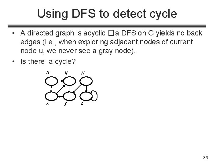
Using DFS to detect cycle • A directed graph is acyclic �a DFS on G yields no back edges (i. e. , when exploring adjacent nodes of current node u, we never see a gray node). • Is there a cycle? u v w x y z 36

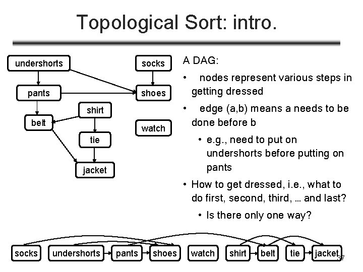
Topological Sort: intro. undershorts socks pants A DAG: • nodes represent various steps in getting dressed • edge (a, b) means a needs to be done before b shoes shirt belt watch tie jacket • e. g. , need to put on undershorts before putting on pants • How to get dressed, i. e. , what to do first, second, third, … and last? • Is there only one way? socks undershorts pants shoes watch shirt belt tie jacket 37

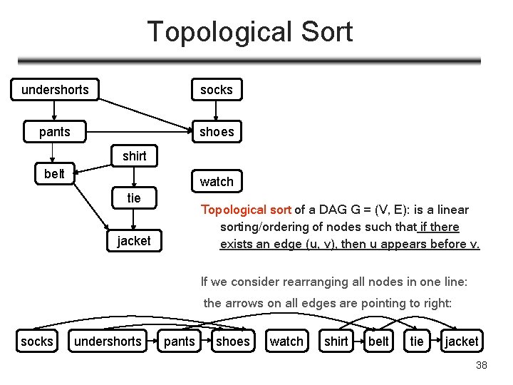
Topological Sort undershorts socks pants shoes shirt belt watch tie Topological sort of a DAG G = (V, E): is a linear sorting/ordering of nodes such that if there exists an edge (u, v), then u appears before v. jacket If we consider rearranging all nodes in one line: the arrows on all edges are pointing to right: socks undershorts pants shoes watch shirt belt tie jacket 38

Topological Sort Algorithm • Given a DAG G=(V, E): • Output: Topological ordering of nodes such that if there exists an edge (u, v), then u appears before v. • Brute force way? undershorts socks pants shoes shirt belt watch tie jacket 39

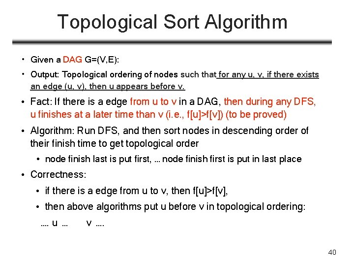
Topological Sort Algorithm • Given a DAG G=(V, E): • Output: Topological ordering of nodes such that for any u, v, if there exists an edge (u, v), then u appears before v. • Fact: If there is a edge from u to v in a DAG, then during any DFS, u finishes at a later time than v (i. e. , f[u]>f[v]) (to be proved) • Algorithm: Run DFS, and then sort nodes in descending order of their finish time to get topological order • node finish last is put first, … node finish first is put in last place • Correctness: • if there is a edge from u to v, then f[u]>f[v], • then above algorithms put u before v in topological ordering: …. u … v …. 40

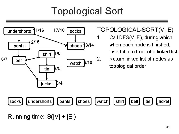
Topological Sort undershorts 11/16 pants 6/7 17/18 socks TOPOLOGICAL-SORT(V, E) 1. 12/15 shoes 13/14 shirt 1/8 belt watch 9/10 tie 2. 2/5 Call DFS(V, E), during which when each node is finished, insert it into front of a linked list Return linked list of nodes as topological order jacket 3/4 socks undershorts pants shoes watch shirt belt tie jacket Running time: Θ(|V| + |E|) 41

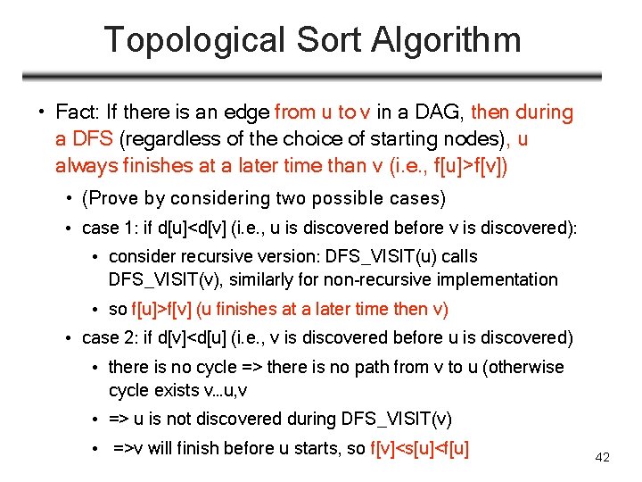
Topological Sort Algorithm • Fact: If there is an edge from u to v in a DAG, then during a DFS (regardless of the choice of starting nodes), u always finishes at a later time than v (i. e. , f[u]>f[v]) • (Prove by considering two possible cases) • case 1: if d[u]<d[v] (i. e. , u is discovered before v is discovered): • consider recursive version: DFS_VISIT(u) calls DFS_VISIT(v), similarly for non-recursive implementation • so f[u]>f[v] (u finishes at a later time then v) • case 2: if d[v]<d[u] (i. e. , v is discovered before u is discovered) • there is no cycle => there is no path from v to u (otherwise cycle exists v…u, v • => u is not discovered during DFS_VISIT(v) • =>v will finish before u starts, so f[v]<s[u]<f[u] 42

Summary • Graph everywhere: represent binary relation • Graph Representation • Adjacent lists, Adjacent matrix • Path, Cycle, Tree, Connectivity • Graph Traversal Algorithm: systematic way to explore graph (nodes) • BFS yields a fat and short tree • • App: find shortest hop path from a node to other nodes DFS yields forest made up of lean and tall tree • App: detect cycles and topological sorting (for DAG) 43