Graph Programming Gordon College 1 Graph Basics A
Graph Programming Gordon College 1
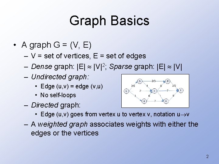
Graph Basics • A graph G = (V, E) – V = set of vertices, E = set of edges – Dense graph: |E| |V|2; Sparse graph: |E| |V| – Undirected graph: • Edge (u, v) = edge (v, u) • No self-loops – Directed graph: • Edge (u, v) goes from vertex u to vertex v, notation u v – A weighted graph associates weights with either the edges or the vertices 2
Representing Graphs • Assume V = {1, 2, …, n} • An adjacency matrix represents the graph as a n x n matrix A: – A[i, j] = 1 if edge (i, j) E (or weight of edge) = 0 if edge (i, j) E – Storage requirements: O(V 2) • Best for a dense representation – But, can be very efficient for small graphs • Especially if stores just one bit per edge • Undirected graph: only need one diagonal of matrix 3
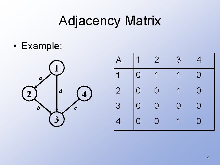
Adjacency Matrix • Example: 1 a d 2 b 4 c 3 A 1 2 3 4 1 0 1 1 0 2 0 0 1 0 3 0 0 4 0 0 1 0 4
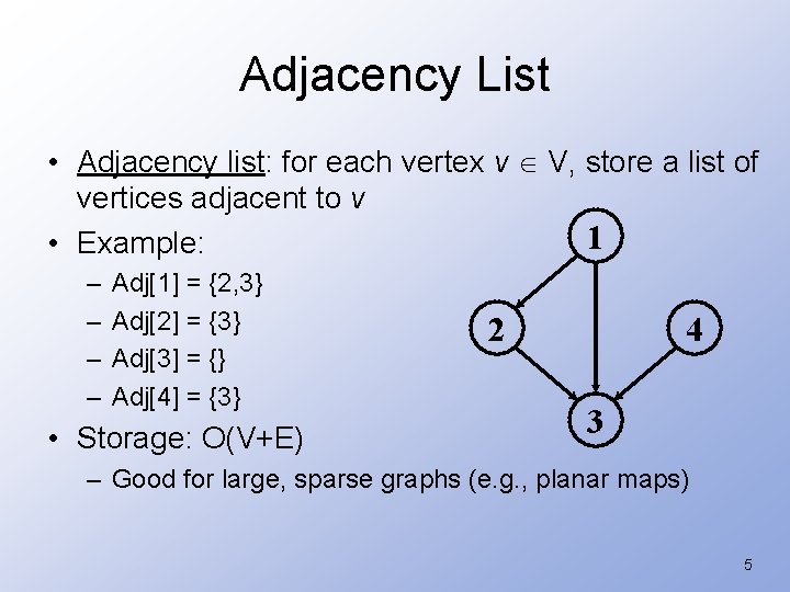
Adjacency List • Adjacency list: for each vertex v V, store a list of vertices adjacent to v 1 • Example: – – Adj[1] = {2, 3} Adj[2] = {3} Adj[3] = {} Adj[4] = {3} • Storage: O(V+E) 2 4 3 – Good for large, sparse graphs (e. g. , planar maps) 5
Graph Searching • Given: a graph G = (V, E), directed or undirected • Goal: methodically explore (visit) every vertex and every edge • Ultimately: build a tree on the graph – Pick a vertex as the root – Choose certain edges to produce a tree – Note: might also build a forest if graph is not connected 6
Breadth-First Search • “Explore” a graph, turning it into a tree – One vertex at a time – Expand frontier of explored vertices across the breadth of the frontier • Builds a tree over the graph – Pick a source vertex to be the root – Find (“discover”) its children, then their children, etc. • Emulates the level-order scan of a binary tree 7
Breadth-First Search • Will associate vertex “colors” to guide the algorithm – White vertices have not been discovered • All vertices start out white – Grey vertices are discovered but not fully explored • They may be adjacent to white vertices – Black vertices are discovered and fully explored • They are adjacent only to black and gray vertices • Explore vertices by scanning adjacency list of grey vertices 8
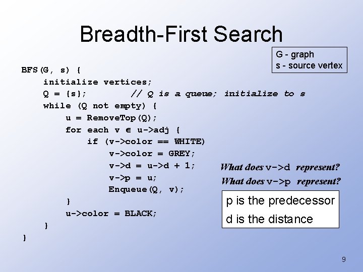
Breadth-First Search G - graph s - source vertex BFS(G, s) { initialize vertices; Q = {s}; // Q is a queue; initialize to s while (Q not empty) { u = Remove. Top(Q); for each v u->adj { if (v->color == WHITE) v->color = GREY; v->d = u->d + 1; What does v->d represent? v->p = u; What does v->p represent? Enqueue(Q, v); } p is the predecessor u->color = BLACK; d is the distance } } 9
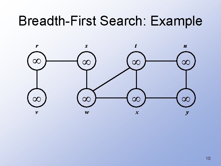
Breadth-First Search: Example r s t u v w x y 10
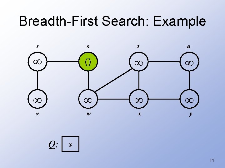
Breadth-First Search: Example r s t u 0 v w x y Q: s 11
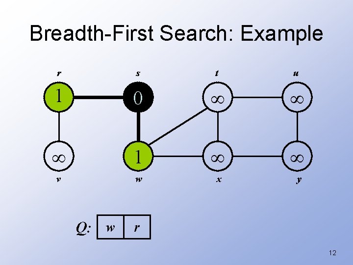
Breadth-First Search: Example r s t u 1 0 1 v w x y Q: w r 12
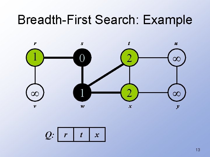
Breadth-First Search: Example r s t u 1 0 2 1 2 v w x y Q: r t x 13
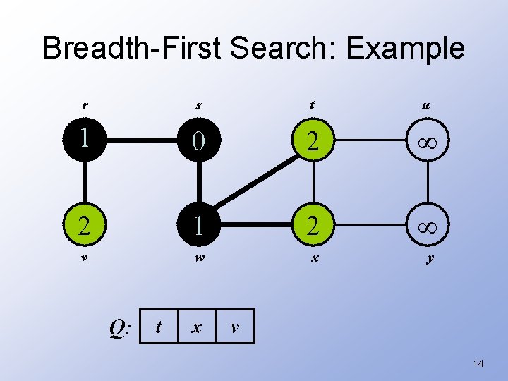
Breadth-First Search: Example r s t u 1 0 2 2 1 2 v w x y Q: t x v 14
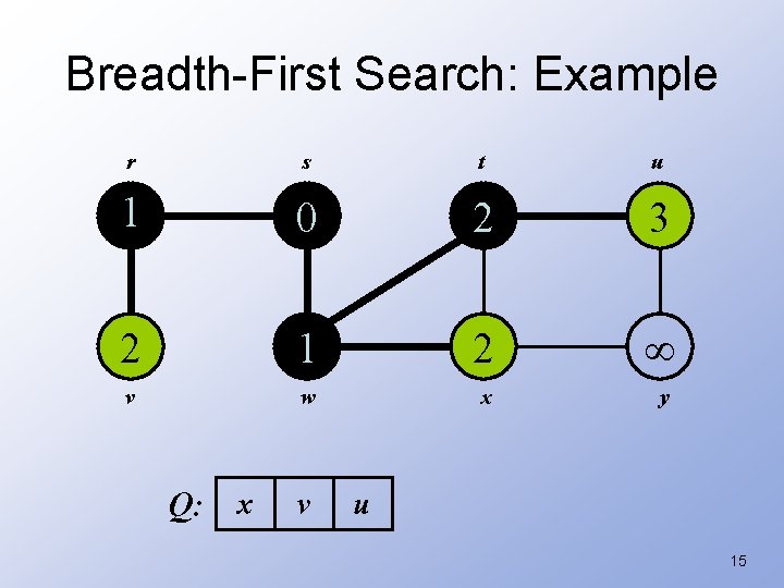
Breadth-First Search: Example r s t u 1 0 2 3 2 1 2 v w x y Q: x v u 15
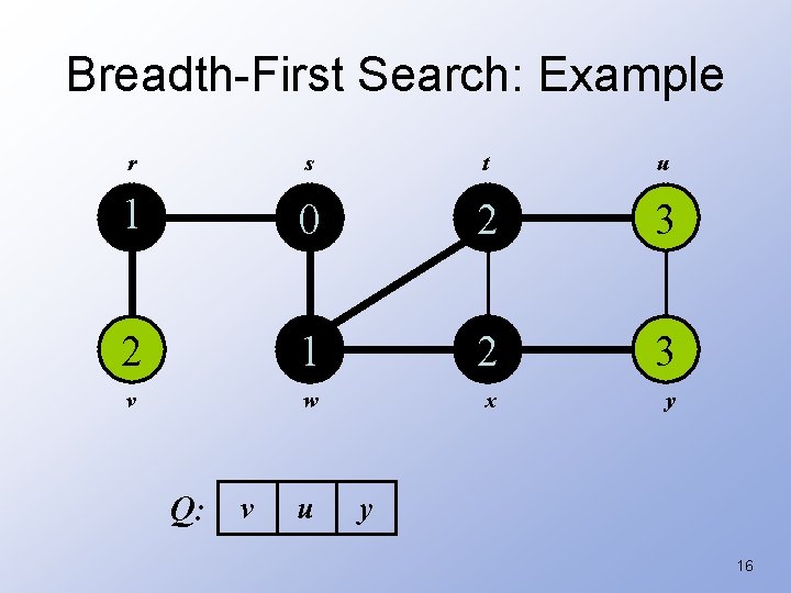
Breadth-First Search: Example r s t u 1 0 2 3 2 1 2 3 v w x y Q: v u y 16
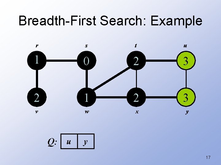
Breadth-First Search: Example r s t u 1 0 2 3 2 1 2 3 v w x y Q: u y 17
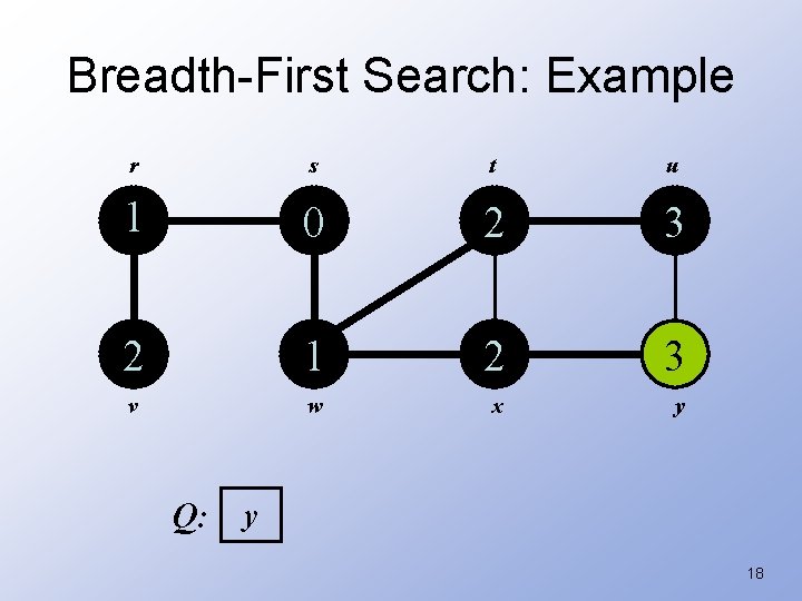
Breadth-First Search: Example r s t u 1 0 2 3 2 1 2 3 v w x y Q: y 18
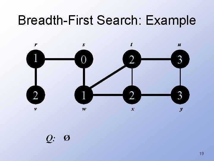
Breadth-First Search: Example r s t u 1 0 2 3 2 1 2 3 v w x y Q: Ø 19
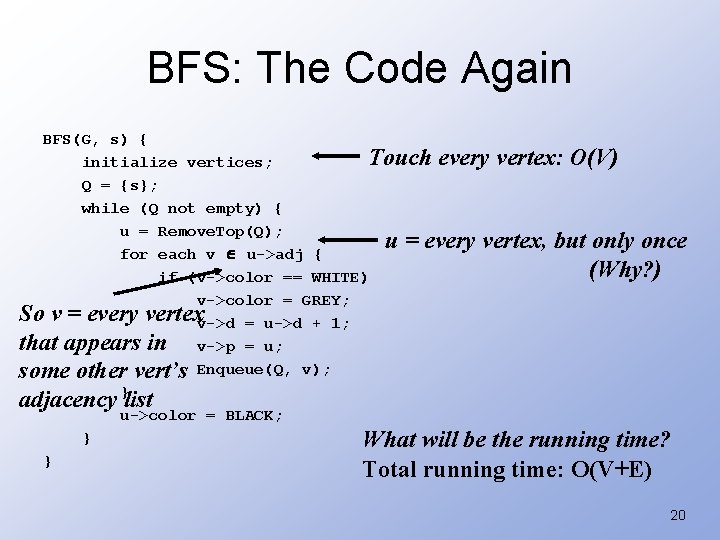
BFS: The Code Again BFS(G, s) { Touch every vertex: O(V) initialize vertices; Q = {s}; while (Q not empty) { u = Remove. Top(Q); u = every vertex, but only once for each v u->adj { (Why? ) if (v->color == WHITE) v->color = GREY; So v = every vertexv->d = u->d + 1; that appears in v->p = u; some other vert’s Enqueue(Q, v); adjacency }list u->color = BLACK; } What will be the running time? } Total running time: O(V+E) 20
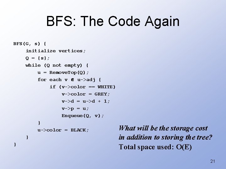
BFS: The Code Again BFS(G, s) { initialize vertices; Q = {s}; while (Q not empty) { u = Remove. Top(Q); for each v u->adj { if (v->color == WHITE) v->color = GREY; v->d = u->d + 1; v->p = u; Enqueue(Q, v); } u->color = BLACK; } } What will be the storage cost in addition to storing the tree? Total space used: O(E) 21
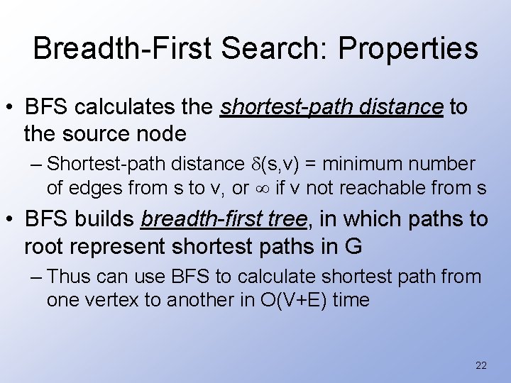
Breadth-First Search: Properties • BFS calculates the shortest-path distance to the source node – Shortest-path distance (s, v) = minimum number of edges from s to v, or if v not reachable from s • BFS builds breadth-first tree, in which paths to root represent shortest paths in G – Thus can use BFS to calculate shortest path from one vertex to another in O(V+E) time 22
Depth-First Search • Depth-first search is another strategy for exploring a graph – Explore “deeper” in the graph whenever possible – Edges are explored out of the most recently discovered vertex v that still has unexplored edges – When all of v’s edges have been explored, backtrack to the vertex from which v was discovered – Emulates the postorder scan of a binary tree 23
Depth-First Search • Vertices initially colored white • Then colored gray when discovered • Then black when finished 24
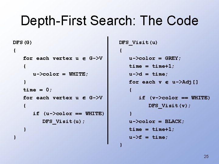
Depth-First Search: The Code DFS(G) { for each vertex u G->V { u->color = WHITE; } time = 0; for each vertex u G->V { if (u->color == WHITE) DFS_Visit(u); } } DFS_Visit(u) { u->color = GREY; time = time+1; u->d = time; for each v u->Adj[] { if (v->color == WHITE) DFS_Visit(v); } u->color = BLACK; time = time+1; u->f = time; } 25
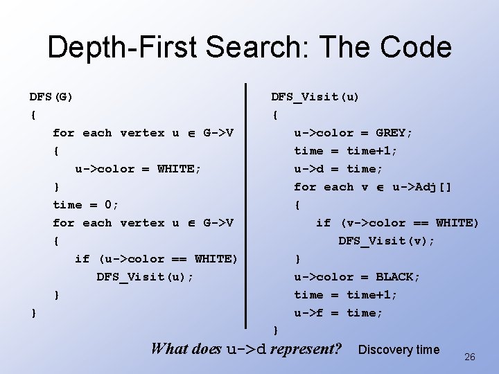
Depth-First Search: The Code DFS(G) { for each vertex u G->V { u->color = WHITE; } time = 0; for each vertex u G->V { if (u->color == WHITE) DFS_Visit(u); } } DFS_Visit(u) { u->color = GREY; time = time+1; u->d = time; for each v u->Adj[] { if (v->color == WHITE) DFS_Visit(v); } u->color = BLACK; time = time+1; u->f = time; } What does u->d represent? Discovery time 26

Depth-First Search: The Code DFS(G) { for each vertex u G->V { u->color = WHITE; } time = 0; for each vertex u G->V { if (u->color == WHITE) DFS_Visit(u); } } DFS_Visit(u) { u->color = GREY; time = time+1; u->d = time; for each v u->Adj[] { if (v->color == WHITE) DFS_Visit(v); } u->color = BLACK; time = time+1; u->f = time; } What does u->f represent? Finishing time 27
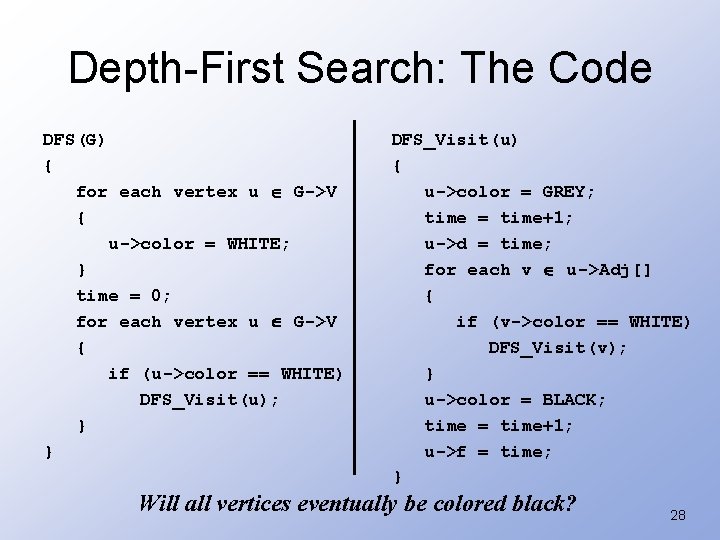
Depth-First Search: The Code DFS(G) { for each vertex u G->V { u->color = WHITE; } time = 0; for each vertex u G->V { if (u->color == WHITE) DFS_Visit(u); } } DFS_Visit(u) { u->color = GREY; time = time+1; u->d = time; for each v u->Adj[] { if (v->color == WHITE) DFS_Visit(v); } u->color = BLACK; time = time+1; u->f = time; } Will all vertices eventually be colored black? 28
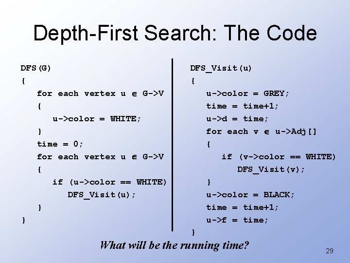
Depth-First Search: The Code DFS(G) { for each vertex u G->V { u->color = WHITE; } time = 0; for each vertex u G->V { if (u->color == WHITE) DFS_Visit(u); } } DFS_Visit(u) { u->color = GREY; time = time+1; u->d = time; for each v u->Adj[] { if (v->color == WHITE) DFS_Visit(v); } u->color = BLACK; time = time+1; u->f = time; } What will be the running time? 29
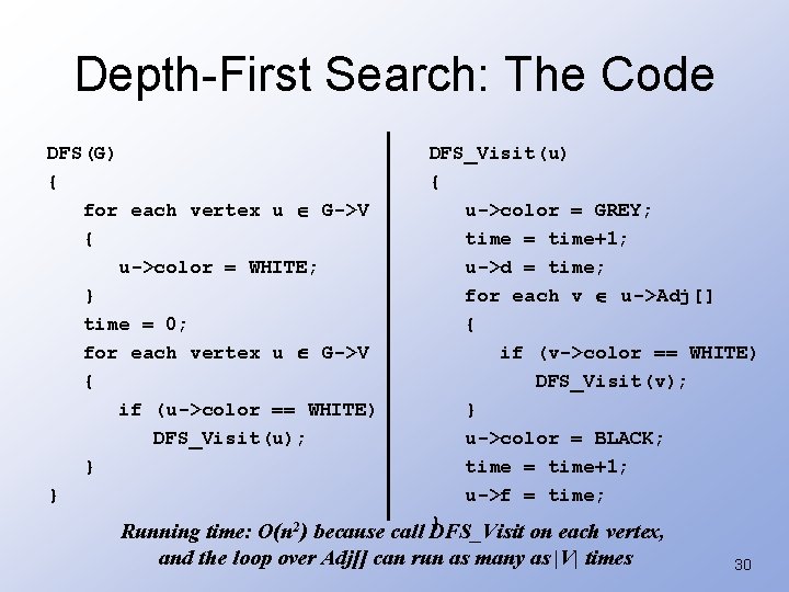
Depth-First Search: The Code DFS(G) { for each vertex u G->V { u->color = WHITE; } time = 0; for each vertex u G->V { if (u->color == WHITE) DFS_Visit(u); } } DFS_Visit(u) { u->color = GREY; time = time+1; u->d = time; for each v u->Adj[] { if (v->color == WHITE) DFS_Visit(v); } u->color = BLACK; time = time+1; u->f = time; } Running time: O(n 2) because call DFS_Visit on each vertex, and the loop over Adj[] can run as many as |V| times 30
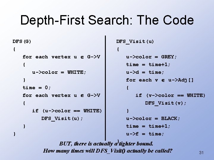
Depth-First Search: The Code DFS(G) { for each vertex u G->V { u->color = WHITE; } time = 0; for each vertex u G->V { if (u->color == WHITE) DFS_Visit(u); } } DFS_Visit(u) { u->color = GREY; time = time+1; u->d = time; for each v u->Adj[] { if (v->color == WHITE) DFS_Visit(v); } u->color = BLACK; time = time+1; u->f = time; BUT, there is actually a}tighter bound. How many times will DFS_Visit() actually be called? 31
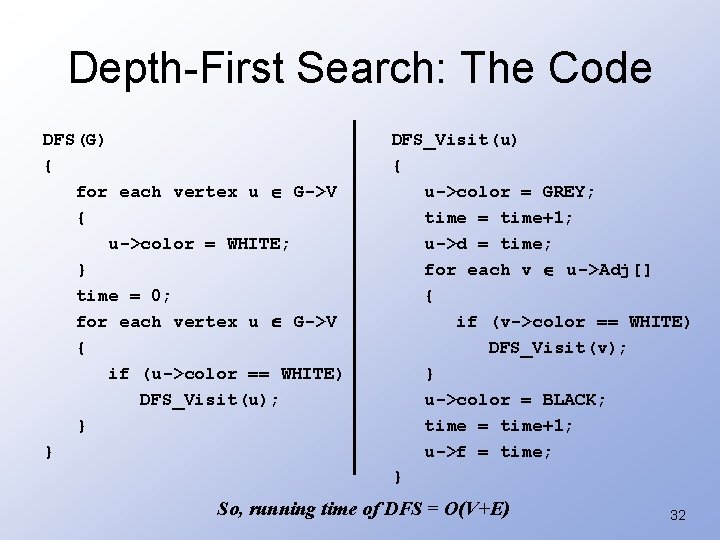
Depth-First Search: The Code DFS(G) { for each vertex u G->V { u->color = WHITE; } time = 0; for each vertex u G->V { if (u->color == WHITE) DFS_Visit(u); } } DFS_Visit(u) { u->color = GREY; time = time+1; u->d = time; for each v u->Adj[] { if (v->color == WHITE) DFS_Visit(v); } u->color = BLACK; time = time+1; u->f = time; } So, running time of DFS = O(V+E) 32
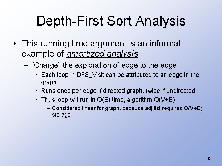
Depth-First Sort Analysis • This running time argument is an informal example of amortized analysis – “Charge” the exploration of edge to the edge: • Each loop in DFS_Visit can be attributed to an edge in the graph • Runs once per edge if directed graph, twice if undirected • Thus loop will run in O(E) time, algorithm O(V+E) – Considered linear for graph, because adj list requires O(V+E) storage 33
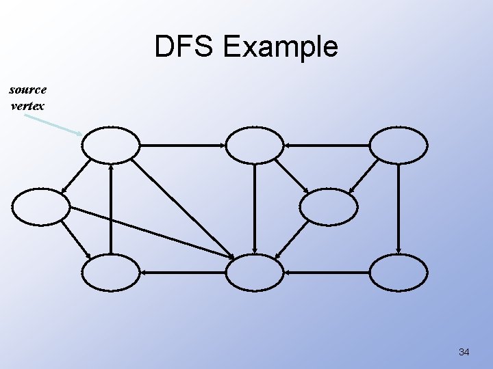
DFS Example source vertex 34
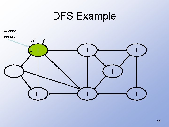
DFS Example source vertex d f 1 | | | | 35
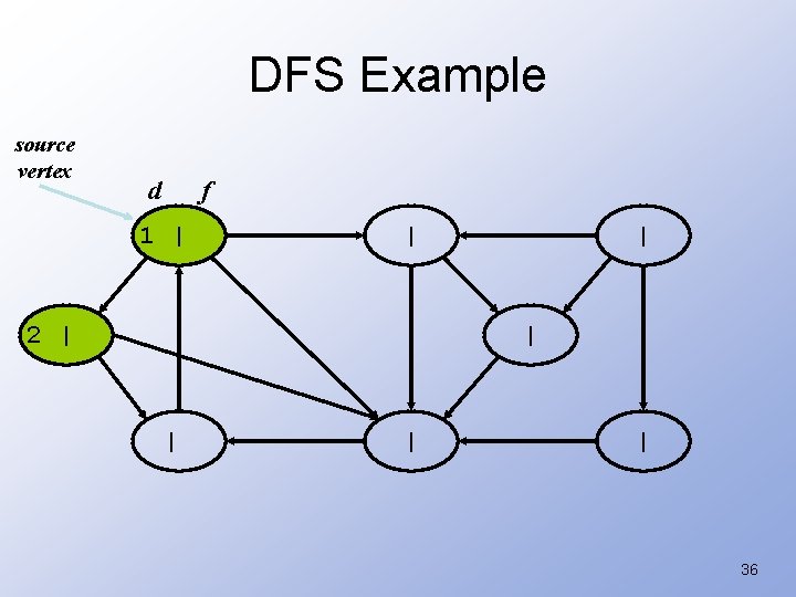
DFS Example source vertex d f 1 | | 2 | | | 36
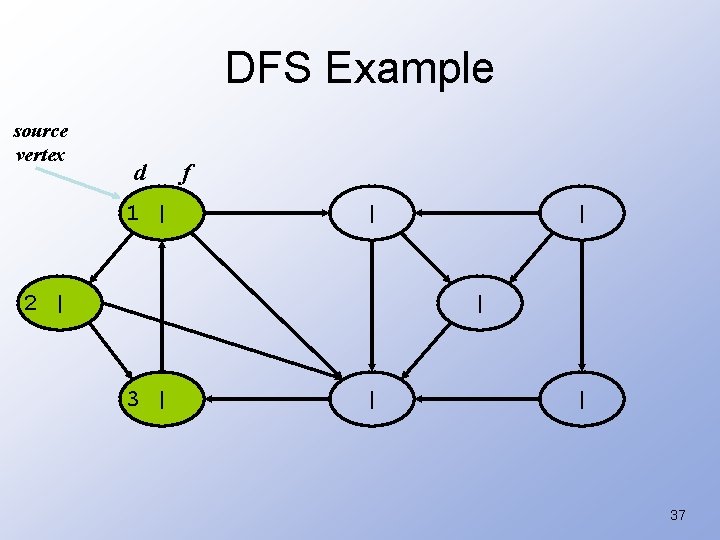
DFS Example source vertex d 1 | f | 2 | | | 37
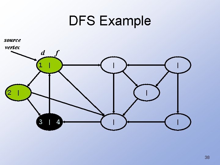
DFS Example source vertex d f 1 | | 2 | | | 3 | 4 | | 38
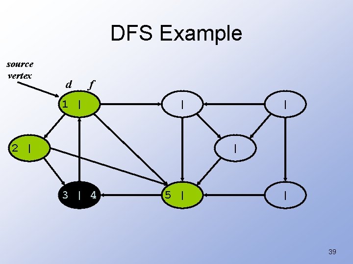
DFS Example source vertex d f 1 | | 2 | | | 3 | 4 5 | | 39
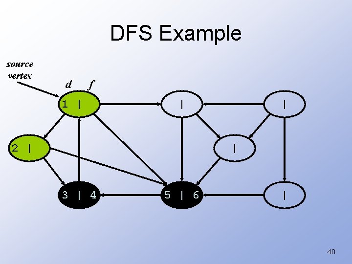
DFS Example source vertex d f 1 | | 2 | | | 3 | 4 5 | 6 | 40
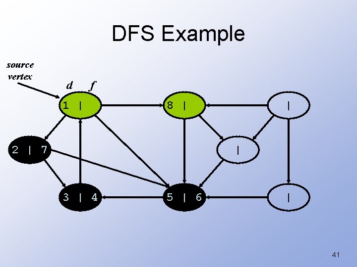
DFS Example source vertex d f 1 | 8 | 2 | 7 | | 3 | 4 5 | 6 | 41

DFS Example source vertex d f 1 | 8 | 2 | 7 | | 3 | 4 5 | 6 | 42
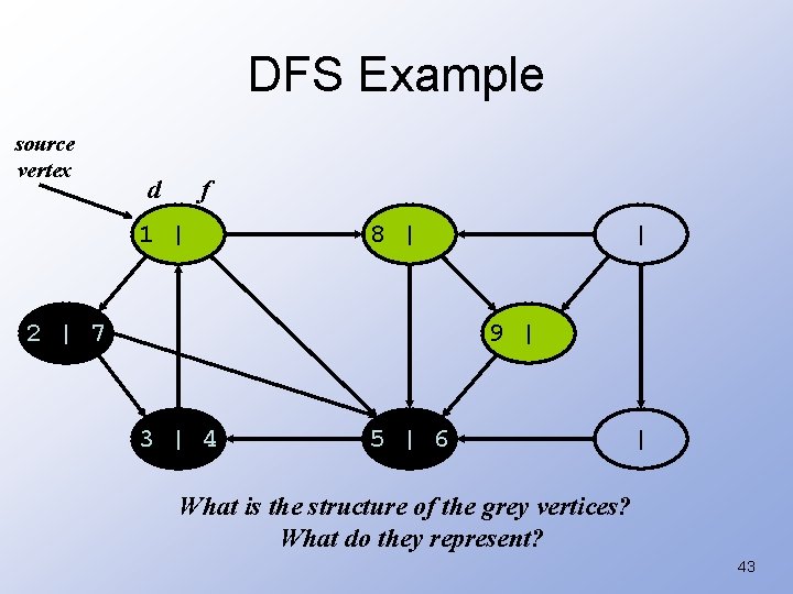
DFS Example source vertex d f 1 | 8 | 2 | 7 | 9 | 3 | 4 5 | 6 | What is the structure of the grey vertices? What do they represent? 43
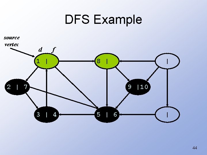
DFS Example source vertex d f 1 | 8 | 2 | 7 | 9 |10 3 | 4 5 | 6 | 44
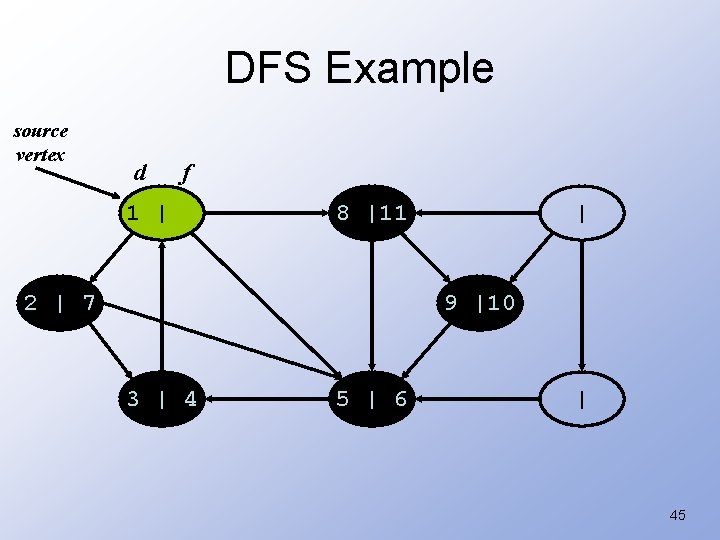
DFS Example source vertex d f 1 | 8 |11 2 | 7 | 9 |10 3 | 4 5 | 6 | 45
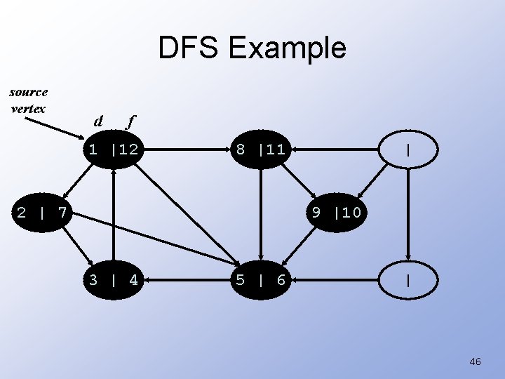
DFS Example source vertex d f 1 |12 8 |11 2 | 7 | 9 |10 3 | 4 5 | 6 | 46
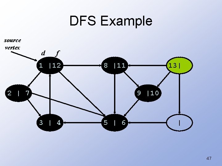
DFS Example source vertex d f 1 |12 8 |11 2 | 7 13| 9 |10 3 | 4 5 | 6 | 47
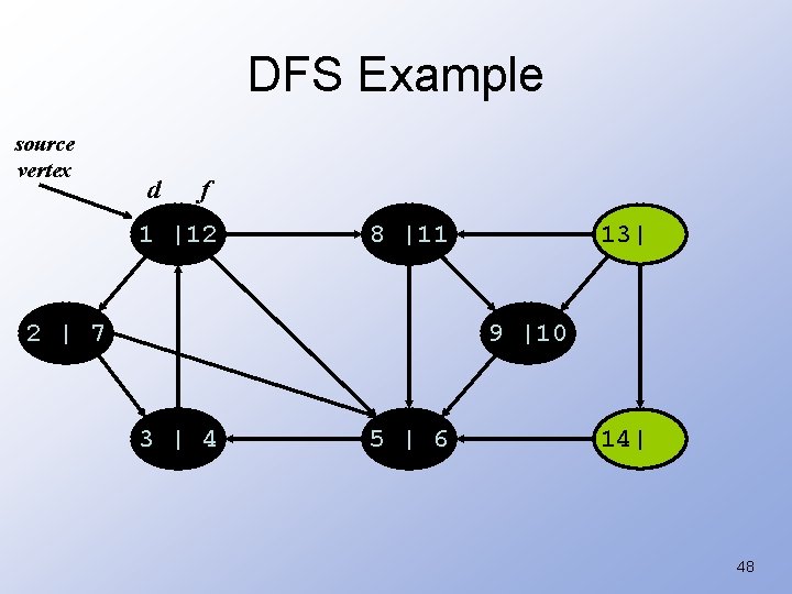
DFS Example source vertex d f 1 |12 8 |11 2 | 7 13| 9 |10 3 | 4 5 | 6 14| 48
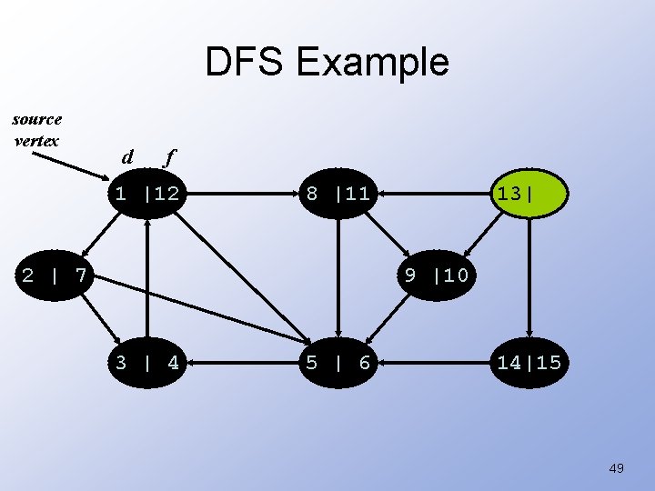
DFS Example source vertex d f 1 |12 8 |11 2 | 7 13| 9 |10 3 | 4 5 | 6 14|15 49
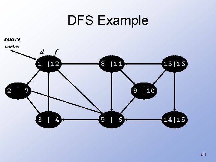
DFS Example source vertex d f 1 |12 8 |11 2 | 7 13|16 9 |10 3 | 4 5 | 6 14|15 50
DFS: Kinds of edges • DFS introduces an important distinction among edges in the original graph: – Tree edge: encounter new (white) vertex • The tree edges form a spanning forest • Can tree edges form cycles? Why or why not? 51
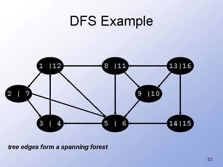
DFS Example 1 |12 8 |11 2 | 7 13|16 9 |10 3 | 4 5 | 6 14|15 tree edges form a spanning forest 52
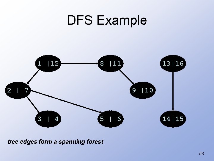
DFS Example 1 |12 8 |11 2 | 7 13|16 9 |10 3 | 4 5 | 6 14|15 tree edges form a spanning forest 53
DFS: Kinds of edges • DFS introduces an important distinction among edges in the original graph: – Tree edge: encounter new (white) vertex – Back edge: from descendent to ancestor • Encounter a grey vertex (grey to grey) 54
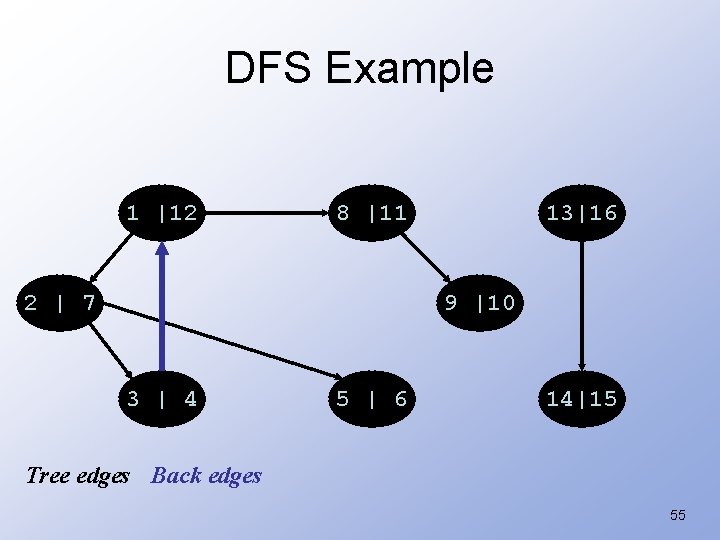
DFS Example 1 |12 8 |11 2 | 7 13|16 9 |10 3 | 4 5 | 6 14|15 Tree edges Back edges 55
DFS: Kinds of edges • DFS introduces an important distinction among edges in the original graph: – Tree edge: encounter new (white) vertex – Back edge: from descendent to ancestor – Forward edge: from ancestor to descendent • Not a tree edge, though • From grey node to black node 56
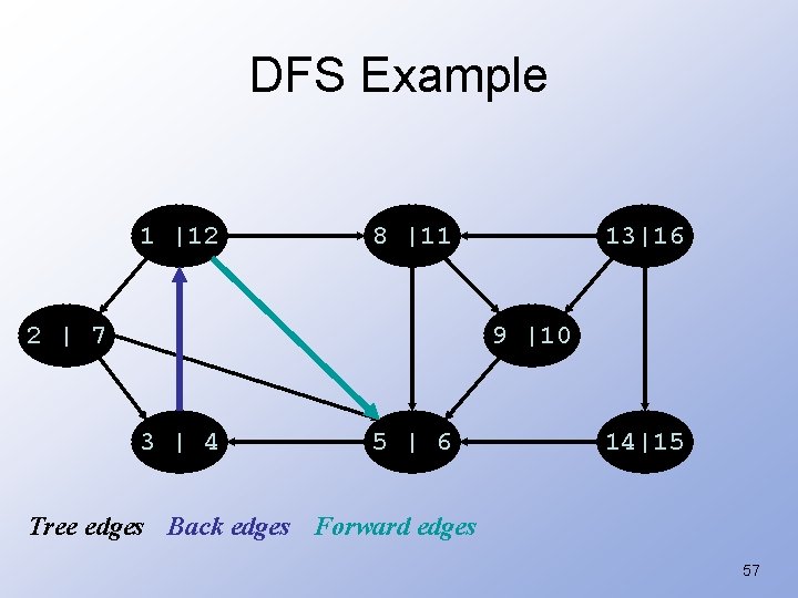
DFS Example 1 |12 8 |11 2 | 7 13|16 9 |10 3 | 4 5 | 6 14|15 Tree edges Back edges Forward edges 57
DFS: Kinds of edges • DFS introduces an important distinction among edges in the original graph: – Tree edge: encounter new (white) vertex – Back edge: from descendent to ancestor – Forward edge: from ancestor to descendent – Cross edge: between a tree or subtrees • From a grey node to a black node 58
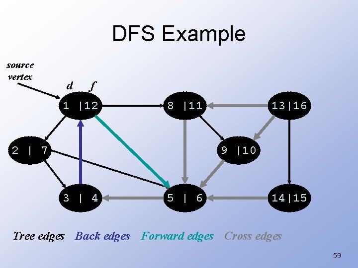
DFS Example source vertex d f 1 |12 8 |11 2 | 7 13|16 9 |10 3 | 4 5 | 6 14|15 Tree edges Back edges Forward edges Cross edges 59
DFS: Kinds of edges • DFS introduces an important distinction among edges in the original graph: – Tree edge: encounter new (white) vertex – Back edge: from descendent to ancestor – Forward edge: from ancestor to descendent – Cross edge: between a tree or subtrees • Note: tree & back edges are important; most algorithms don’t distinguish forward & cross 60
- Slides: 60