Graph Partitioning using Single Commodity Flows Rohit Khandekar

Graph Partitioning using Single Commodity Flows Rohit Khandekar UC Berkeley Joint work with Satish Rao and Umesh Vazirani

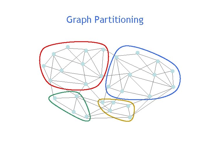
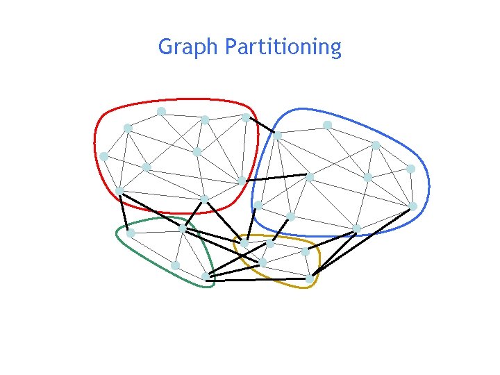
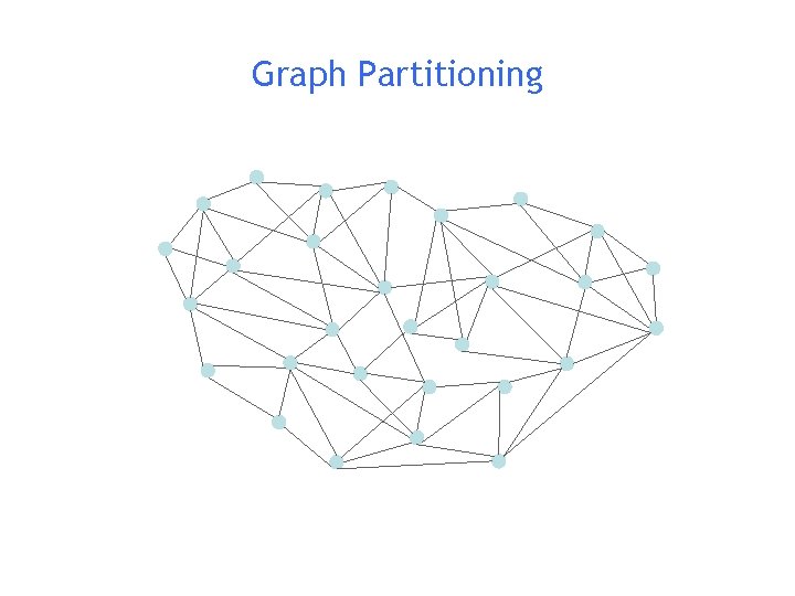
Graph Partitioning

Graph Partitioning

Outline • The sparsest cut problem • Previous work • Our algorithm and outline of analysis • Open questions

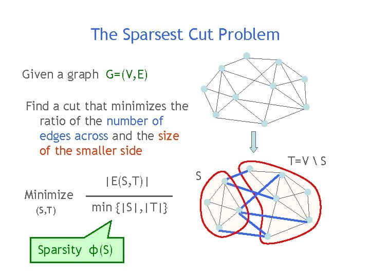
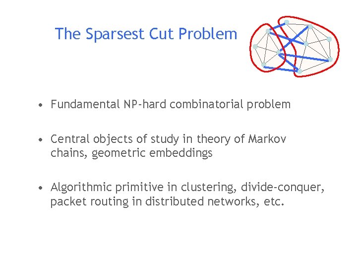
The Sparsest Cut Problem Given a graph G=(V, E) Find a cut that minimizes the ratio of the number of edges across and the size of the smaller side Minimize (S, T) |E(S, T)| min {|S|, |T|} Sparsity ф(S) T=V S S

The Sparsest Cut Problem • Fundamental NP-hard combinatorial problem • Central objects of study in theory of Markov chains, geometric embeddings • Algorithmic primitive in clustering, divide-conquer, packet routing in distributed networks, etc.

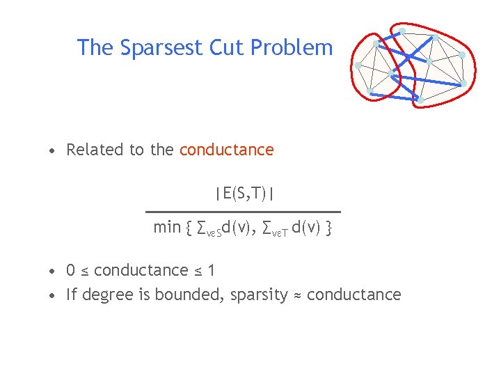
The Sparsest Cut Problem • Related to the conductance |E(S, T)| min { ∑vεSd(v), ∑vεT d(v) } • 0 ≤ conductance ≤ 1 • If degree is bounded, sparsity ≈ conductance

Previous work Three approaches in theory Spectral Method based Multi-Commodity Flow based [Alon-Milman’ 85] [Leighton. Rao’ 88] Semi-definite Programming based [Arora-Rao. Vazirani’ 04] Sparsity = O( ф · log n ) Sparsity = O( ф · √log n ) √ф

Previous work In practice, most successful graph partitioning heuristics use eigenvector based approach, multi-level clustering, max-flows • Chaco [Hendrickson-Leland’ 94] • METIS [Karypis-Kumar’ 98] • Eigenvector + single commodity max-flow [Lang’ 04]

Multi-commodity Flows Send flow between multiple source-sink pairs simultaneously Examples: • Leighton-Rao send flow between every pair of vertices (embed complete graph) • Arora-Rao-Vazirani generalize this approach to embedding an expander graph Computing multi-commodity flows (currently) takes Ω(n 2) time (n = # vertices) even approximately

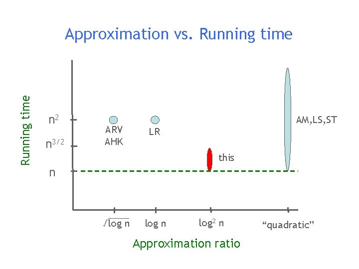
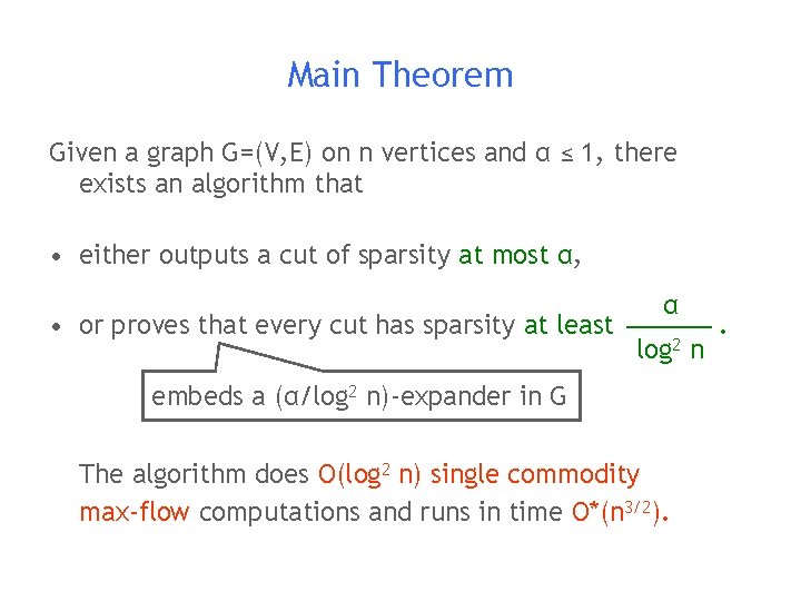
Question Can we get good approximations using a few single commodity flow computations? Answer: YES There exists an algorithm that finds a O(log 2 n) approximation using O(log 2 n) single commodity max-flow computations. It runs in time O*(n 3/2).

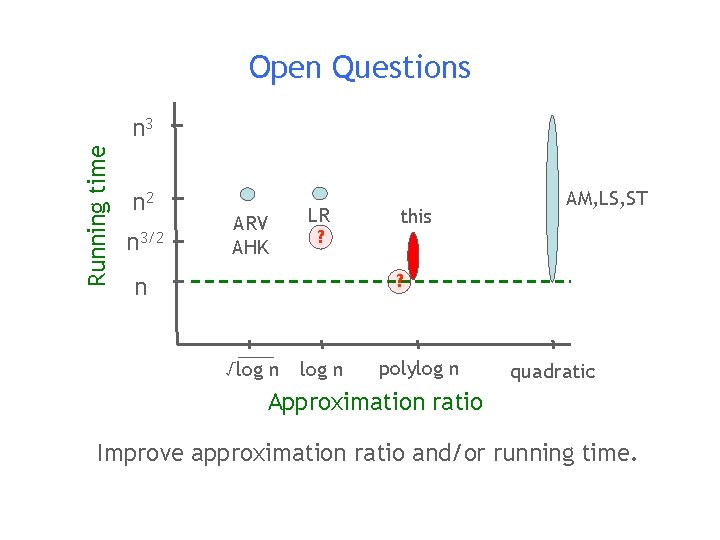
Running time Approximation vs. Running time n 2 n 3/2 ARV AHK AM, LS, ST LR this n √log n log 2 n Approximation ratio “quadratic”

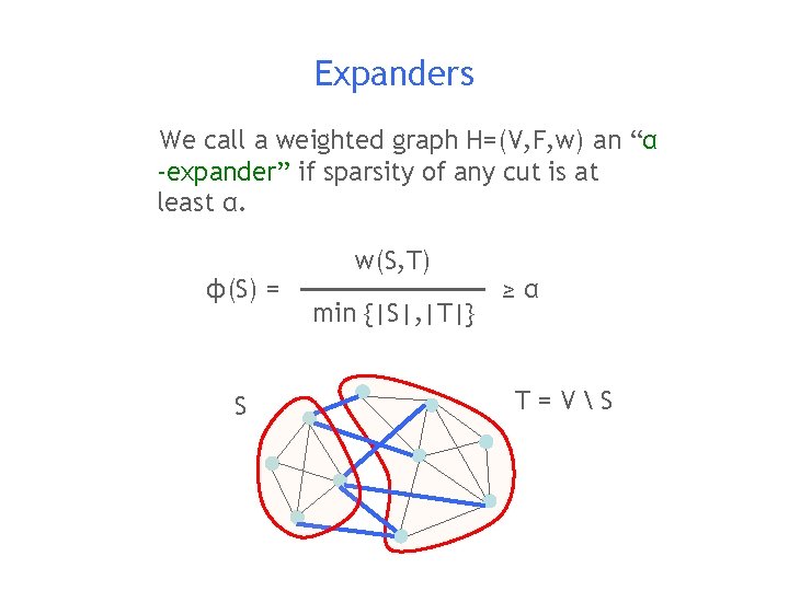
Expanders We call a weighted graph H=(V, F, w) an “α -expander” if sparsity of any cut is at least α. ф(S) = S w(S, T) min {|S|, |T|} ≥α T=VS

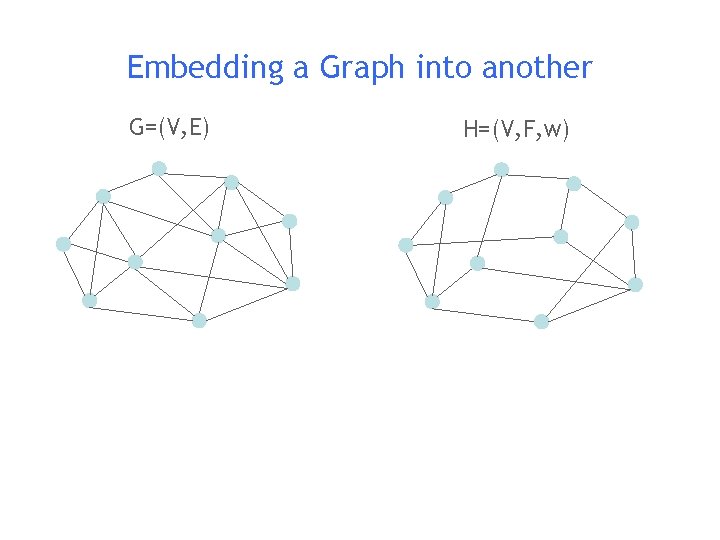
Embedding a Graph into another G=(V, E) H=(V, F, w)

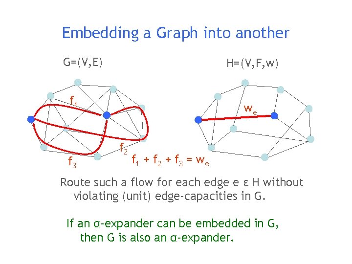
Embedding a Graph into another G=(V, E) H=(V, F, w) f 1 f 3 we f 2 f 1 + f 2 + f 3 = w e Route such a flow for each edge e ε H without violating (unit) edge-capacities in G. If an α-expander can be embedded in G, then G is also an α-expander.

Main Theorem Given a graph G=(V, E) on n vertices and α ≤ 1, there exists an algorithm that • either outputs a cut of sparsity at most α, • or proves that every cut has sparsity at least α log 2 embeds a (α/log 2 n)-expander in G The algorithm does O(log 2 n) single commodity max-flow computations and runs in time O*(n 3/2). n .

Algorithm

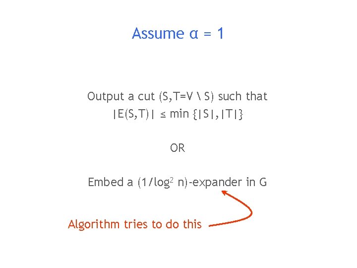
Assume α = 1 Output a cut (S, T=V S) such that |E(S, T)| ≤ min {|S|, |T|} OR Embed a (1/log 2 n)-expander in G Algorithm tries to do this

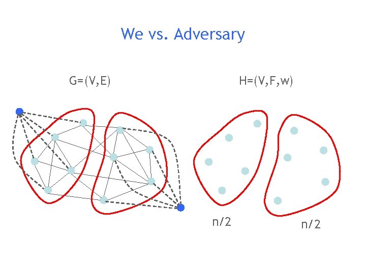
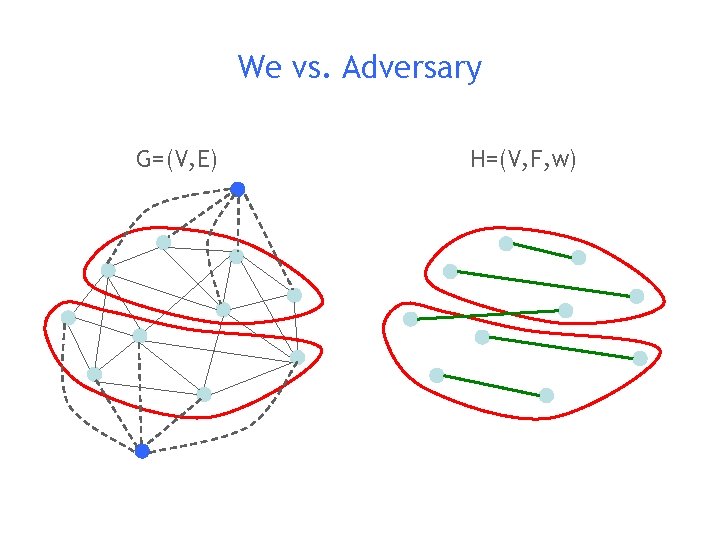
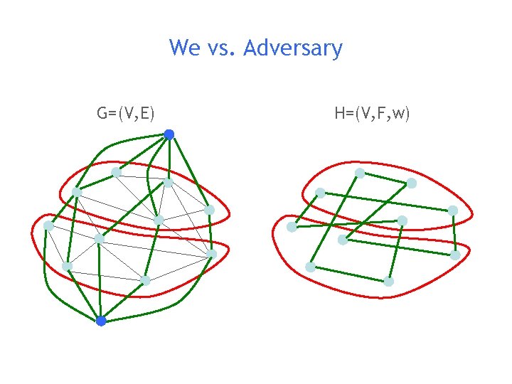
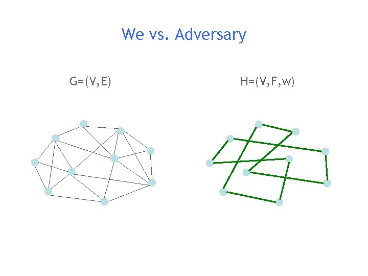
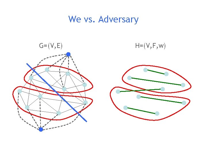
We vs. Adversary H=(V, F, w) G=(V, E) n/2

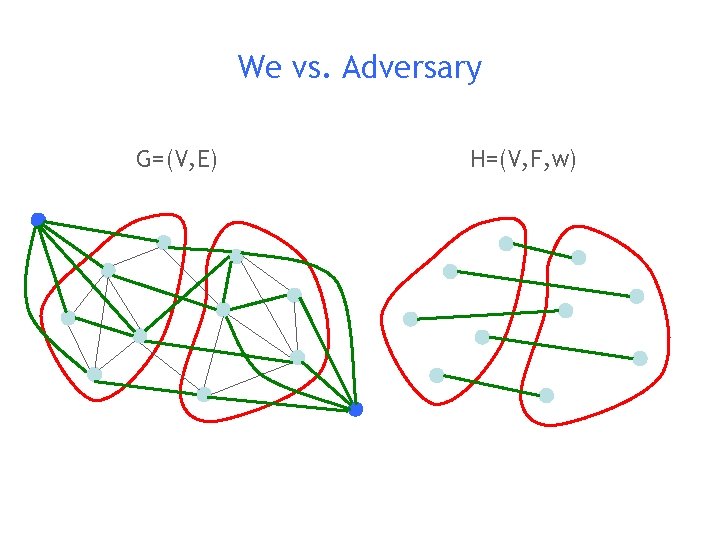
We vs. Adversary G=(V, E) H=(V, F, w)

We vs. Adversary G=(V, E) H=(V, F, w)

We vs. Adversary G=(V, E) H=(V, F, w)

We vs. Adversary G=(V, E) H=(V, F, w)

We vs. Adversary G=(V, E) H=(V, F, w)

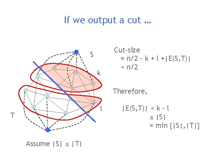
If we output a cut … S k Cut-size = n/2 – k + l +|E(S, T)| < n/2 Therefore, l T Assume |S| ≤ |T| |E(S, T)| < k – l ≤ |S| = min {|S|, |T|}

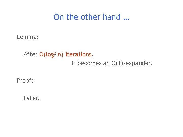
On the other hand … Lemma: After O(log 2 n) iterations, H becomes an Ω(1)-expander. Proof: Later.

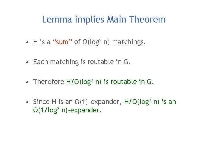
Lemma implies Main Theorem • H is a “sum” of O(log 2 n) matchings. • Each matching is routable in G. • Therefore H/O(log 2 n) is routable in G. • Since H is an Ω(1)-expander, H/O(log 2 n) is an Ω(1/log 2 n)-expander.

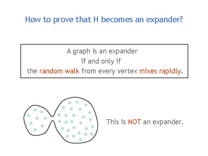
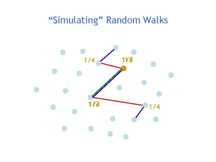
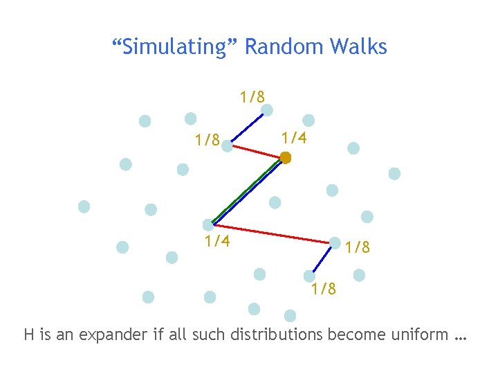
How to prove that H becomes an expander? A graph is an expander if and only if the random walk from every vertex mixes rapidly. This is NOT an expander.

“Simulating” Random Walks 1/4 1/2 1/4 1 1/2 1/4

“Simulating” Random Walks 1/8 1/4 1/8 H is an expander if all such distributions become uniform …

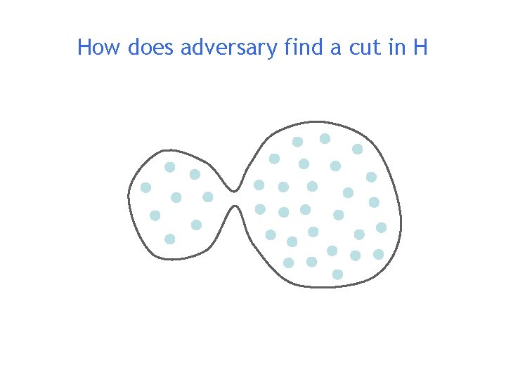
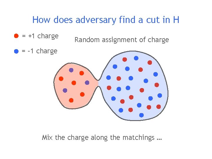
How does adversary find a cut in H Adversary would like to find a balanced cut across which very small amount of probability has crossed over.

How does adversary find a cut in H

How does adversary find a cut in H = +1 charge Random assignment of charge = – 1 charge Mix the charge along the matchings …

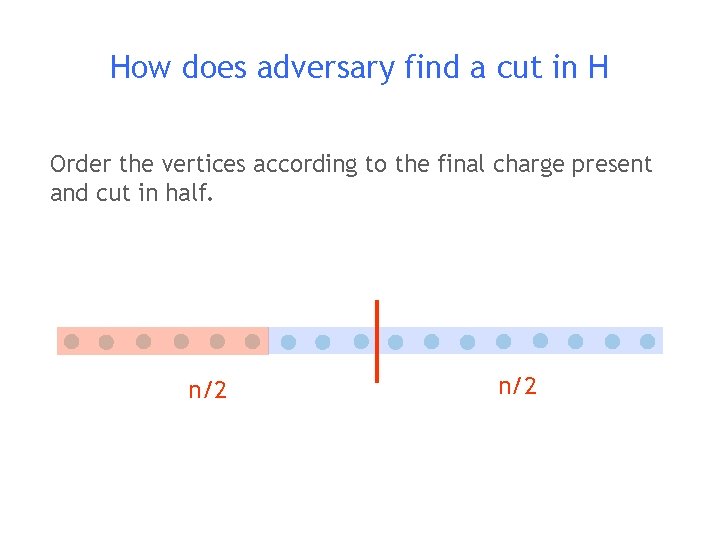
How does adversary find a cut in H Order the vertices according to the final charge present and cut in half. n/2

Analysis

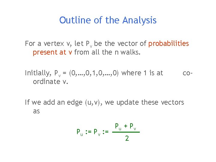
Outline of the Analysis For a vertex v, let Pv be the vector of probabilities present at v from all the n walks. Initially, Pv = (0, …, 0, 1, 0, …, 0) where 1 is at ordinate v. co- If we add an edge (u, v), we update these vectors as Pu : = Pv : = Pu + Pv 2

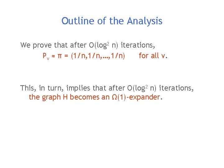
Outline of the Analysis We prove that after O(log 2 n) iterations, Pv ≈ π = (1/n, …, 1/n) for all v. This, in turn, implies that after O(log 2 n) iterations, the graph H becomes an Ω(1)-expander.

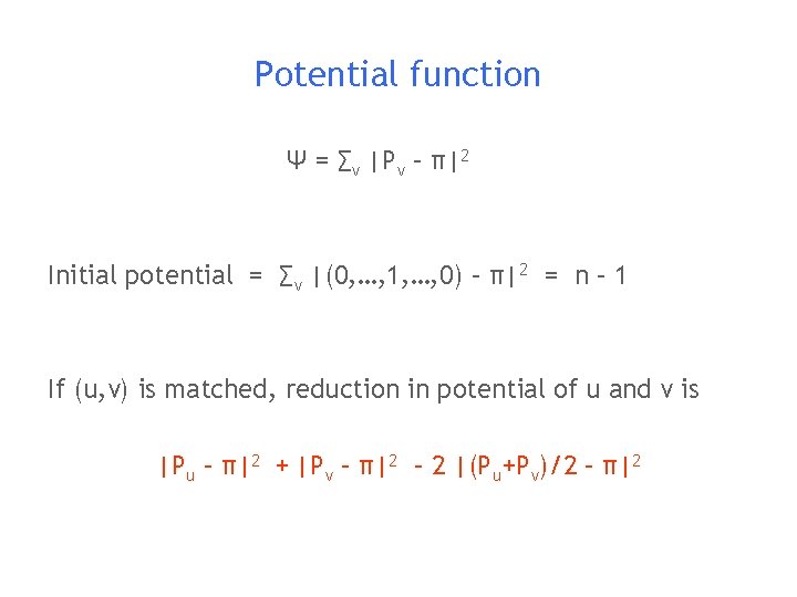
Potential function Ψ = ∑v |Pv – π|2 Initial potential = ∑v |(0, …, 1, …, 0) – π|2 = n – 1 If (u, v) is matched, reduction in potential of u and v is |Pu – π|2 + |Pv – π|2 – 2 |(Pu+Pv)/2 – π|2

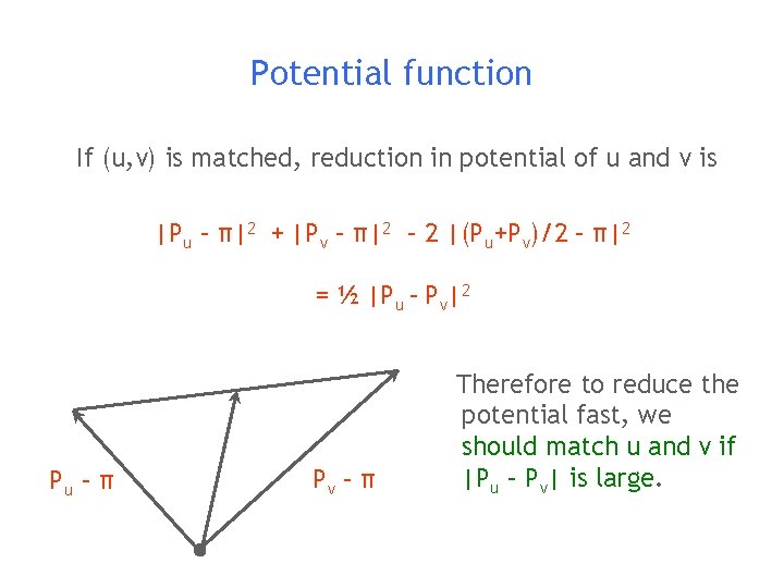
Potential function If (u, v) is matched, reduction in potential of u and v is |Pu – π|2 + |Pv – π|2 – 2 |(Pu+Pv)/2 – π|2 = ½ |Pu – Pv|2 Pu – π Pv – π Therefore to reduce the potential fast, we should match u and v if |Pu – Pv| is large.

Random Projections

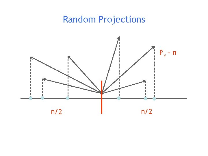
Random Projections Pv – π n/2

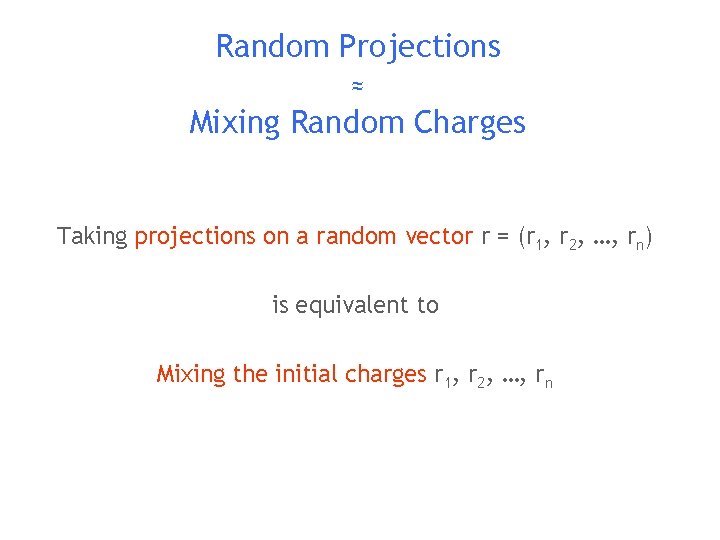
Random Projections ≈ Mixing Random Charges Taking projections on a random vector r = (r 1, r 2, …, rn) is equivalent to Mixing the initial charges r 1, r 2, …, rn

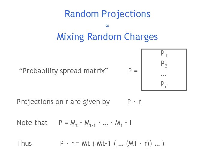
Random Projections ≈ Mixing Random Charges “Probability spread matrix” P= Projections on r are given by P·r P 1 P 2 … Pn Note that P = Mt · Mt-1 · … · M 1 · I Thus P · r = Mt ( Mt-1 ( … (M 1 · r)) … )

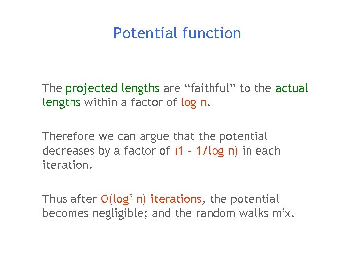
Potential function The projected lengths are “faithful” to the actual lengths within a factor of log n. Therefore we can argue that the potential decreases by a factor of (1 – 1/log n) in each iteration. Thus after O(log 2 n) iterations, the potential becomes negligible; and the random walks mix.

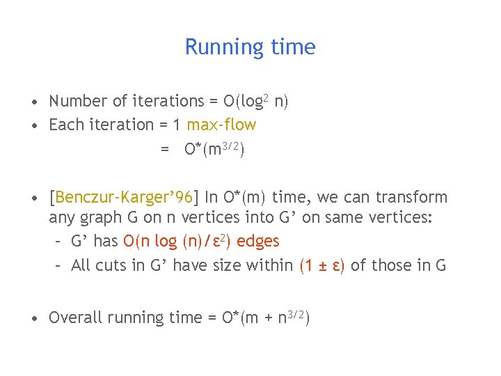
Running time • Number of iterations = O(log 2 n) • Each iteration = 1 max-flow = O*(m 3/2) • [Benczur-Karger’ 96] In O*(m) time, we can transform any graph G on n vertices into G’ on same vertices: – G’ has O(n log (n)/ε 2) edges – All cuts in G’ have size within (1 ± ε) of those in G • Overall running time = O*(m + n 3/2)

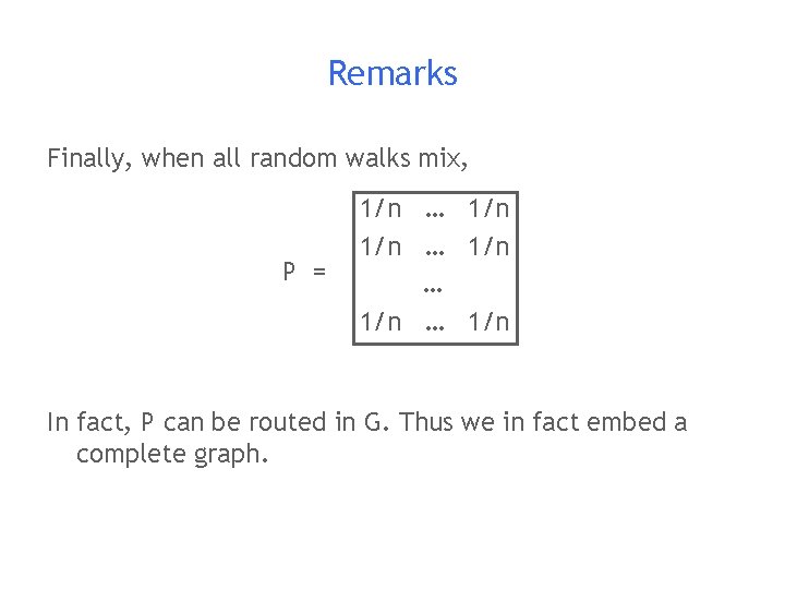
Remarks Finally, when all random walks mix, P = 1/n … 1/n In fact, P can be routed in G. Thus we in fact embed a complete graph.

Extensions to Balanced Separator • Balanced Separator: Partition V into S and T = V S such that – |S|, |T| ≥ n/3, and – |E(S, T)| is minimized. • The techniques can be extended to yield O(log 2 n) approximation for this problem in similar running times.

Open Questions Running time n 3 n 2 n 3/2 ARV AHK LR ? this AM, LS, ST ? n √log n polylog n quadratic Approximation ratio Improve approximation ratio and/or running time.

Open Questions Our algorithm can be thought of as a “primal”“dual” algorithm. Is there a more general framework? Can we extend this technique to other problems?

Thank You

Graph Partitioning